


Time series
A time series is a collection of values of a variable over time:
where can be regularly or irregularly spaced. Most of the literature assumes discrete regularly sampled time series.
Time series patterns
Time series can be characterized by:
Trends: a tendency, a long term change in the mean level
Seasonalities: patterns with constant period lengths
Ciclicities: cyclic patterns with variable lengths
Regime switches / turning points: different trends within a series
Can you spot some of the above features in the following TS plots?
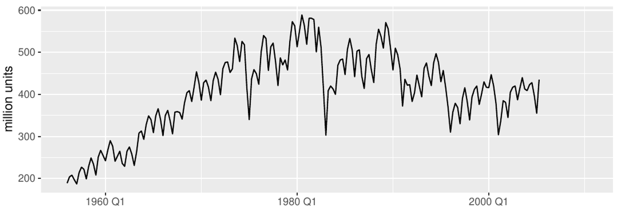
Australian clay brick production
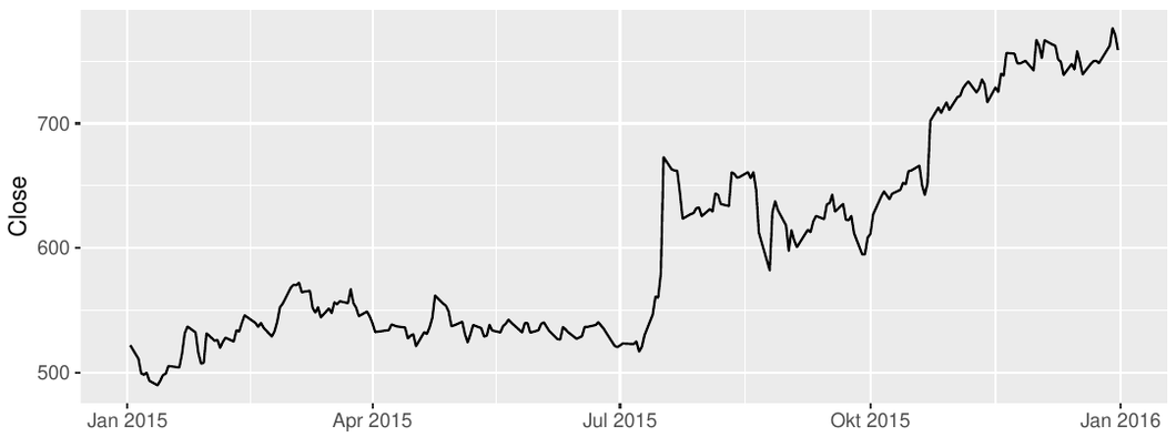
Google closing stock prices
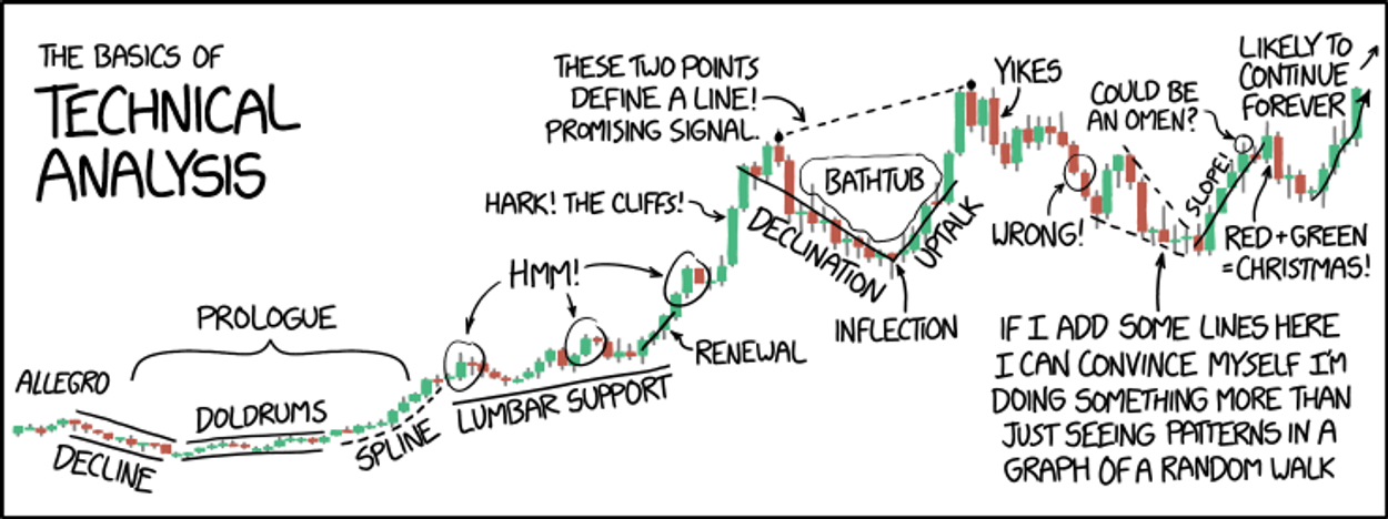
Seek and you will find
What can be forecasted?
Given a pool of signal, which ones can be easily forecasted?
Dual question: Which signals should I give up forecasting?
The single most important conditions in forecasting a time series:

The future is similar to the past
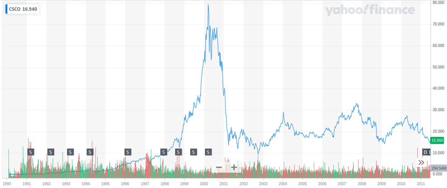
Counterexample: CISCO stock prices between 2000 and 2002
Good news!
In many cases, this condition holds. If it doesn’t, we can try to force it:
remove cycles and trends
remove effect of the forecast on the signal
transform the data
Good news pt. II
We have some tools that help understand whether a given time series is forecastable. These tools are based on a stochastic process representation of time series.
Stochastic processes
A probability space is a triple , where
is a nonempty set, we call it the sample space.
is a σ-algebra of subsets of , i.e. a family of subsets closed
with respect to countable union and complement with respect to
.
is a probability measure defined for all members of ,. That
is a function such that for all ,
, for all sequences
A stochastic process is a family of random variables defined on the same probability space :
Examples
Joint distribution
The joint distribution function of can be defined as:
The above expression is known also as a copula, that is, a cumulative density function over a multivariate space.
If was known for a particular stochastic process , we could answer questions such as:
Which is the probability that the process passes through [a, b] at time ?
Which is the probability that the process passes through [a, b] at time and through [c, d] at time ?
It turns out that this ability is pretty much all we need to know about the stochastic process.
Theorem
Under general conditions the probabilistic structure of the stochastic process is completely specified if we are given the joint probability distribution of for all values of s and for all choices of
(Priestly 1981, p.104)
In fact, once is known, we can generate an infinite set of realizations from the stochastic process , also called scenarios
7 days ahead forecast of the power consumption of a distribution system operator. Blue: observed. Violet: point forecast and possible scenarios
If the future is not similar to the past, we cannot estimate for arbitrary values of s. Even for a univariate stochastic process , this requires to estimate
To reduce the number of parameters to be learned (in the example above ), some regularity conditions must hold.
the TS must be somehow homogeneous in time
the process must have limited memory
Let’s do a step back and try to ask a somehow simpler question:
Is it possible to estimate statistical moments of the time series?
Mean, covariance and where to find them
We define the mean and (auto)covariance of a stochastic process as:
Since we can only observe one realization of the stochastic process in time, estimates for mean and variance can only be done by time averaging (as opposed to sample path average).
Stationary processes and ergodicity
A process is said to be stationary (in a given window) if sliding along the time axis the joint CDF doesn’t change
Additionally, a process is said to be ergodic w.r.t. one of its moment if we can estimate them by observing a sufficiently long realization of the process and if estimations converge quadratically to the true values.
In other words, imagine to observe a set of sample paths . The process is ergodic if averaging over different gets the same results of averaging over time.
Which one of the two examples of stochastic processes above is ergodic?Slutsky’s Theorem
Let be a stationary process with mean and autocovariance
If:
or
then is mean-ergodic
Intuitively, this result tell us that if any two random variables positioned far apart in the sequence are almost uncorrelated, then some new information can be continually added so that the sample mean will approach the population mean.
By the law of large numbers, good estimates of mean and covariance for ergodic processes are:
Beware! In some cases these estimations do not converge quickly
Consider the case in which the stochastic process has distribution:
This is known as Pareto distribution, which is a power law distribution. These are also known as fat tail distributions. Two notable examples of fat-tailed natural variables are earthquakes and pandemics.
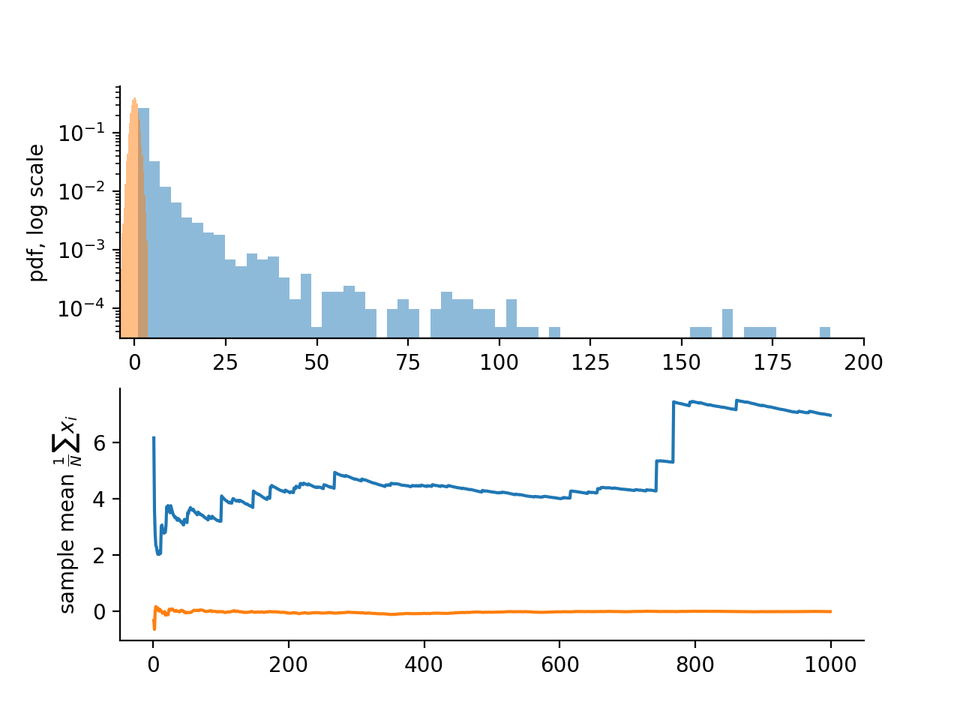
Top: pdfs for normal and pareto distribution with alpha = 1.12. Bottom: convergence of sample means
ACF function
The autocorrelation function is defined as:
If we get only T timesteps to evaluate , we must be careful to keep large enough for the estimation to be meaningful
When evaluating ACF for lag 9 we just got 2 observations to estimate the correlation for a 20-steps time series
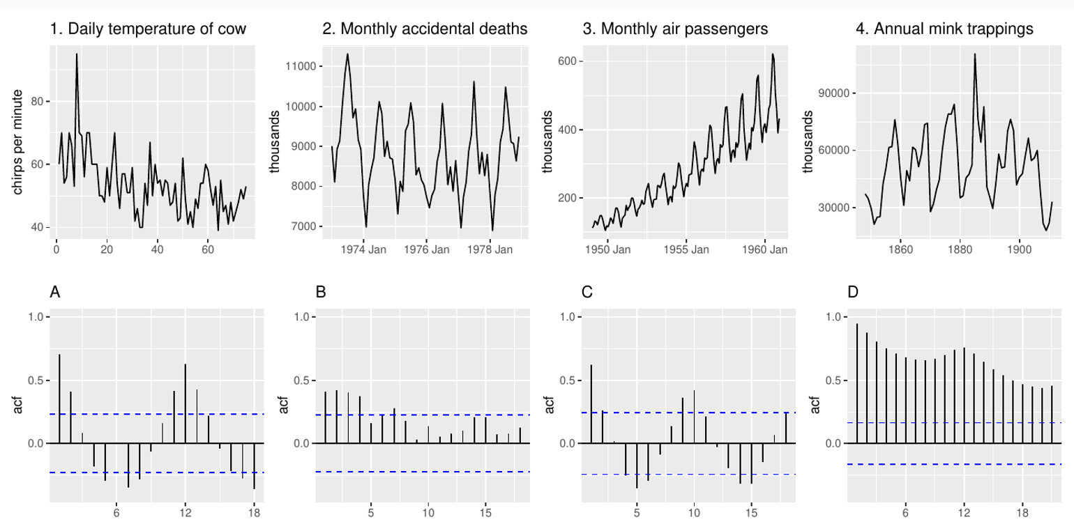
Which is which?
ACF as an IID test
The ACF function can be used to construct the following hypothesis test:
if a process is IID, we have that .
A decision rule for the hypothesis test could be:
reject if
that is, for a given lag we require the magnitude of the correlation to be less than a constant value.
How do we choose c? We can request a 95% confidence level:
We know that for i.i.d. processes for CLT
This means that iff
Why is normally distributed with 0 mean and 1/n variance?
Furthermore, if we call , is still a i.i.d.
Portmanteau tests
Instead of testing a given lag , we can test for a set of lags. For an i.i.d. process, the following random variables are approximately chi-square with K degrees of freedom.
Box-Pierce test
Ljung-Box test
Spectral and approximate entropy
Entropy can be used as a measure of complexity and forecastability. Entropy is a measure of information contained in a random event. Since the information contained in two independent events will sum, while their joint probability is , the only possible form of the information is:
If we take the expected value, and consider events with low probability to be more informative →
Entropy gives an idea of complexity of the distribution of the signal. However, entropy for these two signals will be the same:
[0,1,0,1,0,1,0,1,0,1,0,1,0,1,0,1…] [0,1,1,1,0,0,0,1,0,1,0,0,0,1,0,1, 1,…]
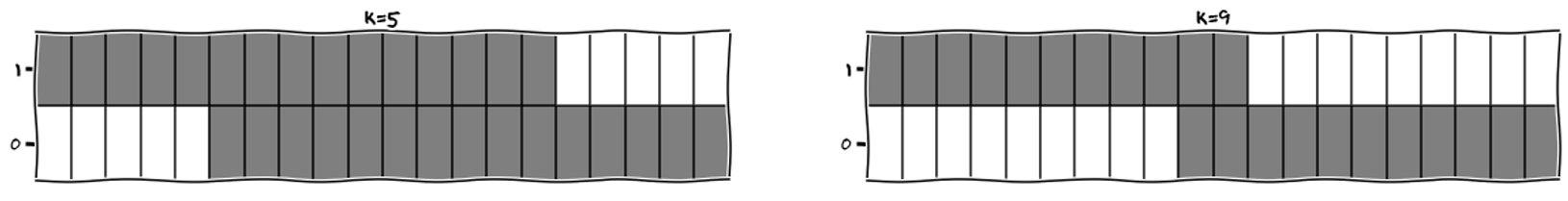
A better measure of forecastability is approximate entropy, which computes the entropy of maximum discrepancy of segments of length m of a time series.
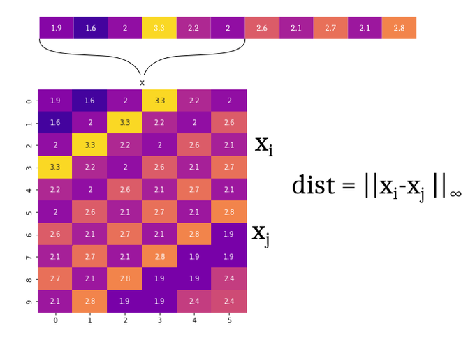
entropy on distribution of “r-close neighbors” of the embedded sequences
Benchmark forecasting methods
Some forecasting methods are extremely simple and yet surprisingly effective. They are stateless methods
Naïve method
This method performs well for , or at scale which are smaller than the characteristic time scale of the signal
Mean method
We just take the mean value of the time series observed so far
Conditional Mean method
We take the mean of the observations that were registered in similar conditions
Example: I’m predicting sales for a given product on an online platform. The platform applies time-varying discounts based on different market conditions. We can forecast the product taking the mean sales in the same day of the week when the same discount was applied.
Seasonal Naïve method
where is the period of the seasonality
Confidence intervals
Assuming residuals are normal, uncorrelated:
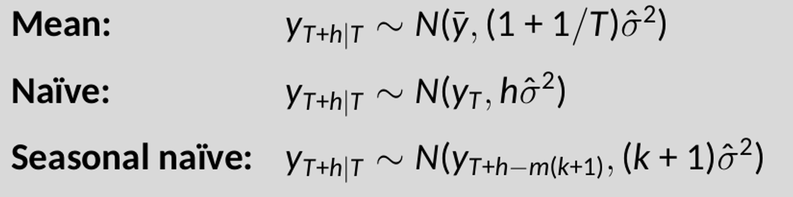
Note that when h=1 and T is large, these all give the same approximate forecast variance
Time series scores
Standard ML metrics are:
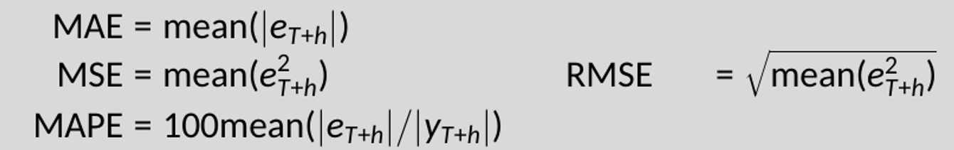
For time series, it is usually better to normalize these scores.
Example: mean absolute scaled error . Here is a normalizing factor.
For non-seasonal time series
is equivalent to MAE relative to a naïve
method.
For seasonal time series
is equivalent to MAE relative to a seasonal
naïve method
Bonus: Confidence intervals derivation
Mean method
The mean model is
Where . For this method, we need to estimate , which is done via empirical mean:
Since the model treats the predicted variable as constant, the prediction error is independent of the step ahead . The predictive distribution is Gaussian, with variance:
The first quantity is the variance associated to the estimation of the parameter , and stems directly from the central limit theorem: the uncertainty in the estimation of the distribution mean through empirical mean is normally distributed with variance ~ (1/T).
Naive method
The naive method assumes that the true data generation process has the following form:
We can obtain the formula for the step ahead prediction as:
Since the errors are considered to be zero mean, the predictive variable and its variance are:
Where the last expression is due to the fact that a summation of Gaussian random variables is still a Gaussian with variance equal to the sum of their variances.
Seasonal method
The seasonal naive method assumes the following datageneration process
This can be rewritten as:
Thus: