


Risk, empirical risk, generalization and fitting strategies
Called out inputs, our target, and their true joint distribution.
If we define as a forecasting model learned by a learning algorithm on adaset ,
model selection is driven by our will to minimize the risk, defined by a loss function :
However, since the true join distribution is unknown, the training process usually involves minimizing the empirical risk on :
 Why minimizing the empirical risk alone is not a good criteria for model selection?
Model selection, generalization error, overfitting
We can state the task of model selection using three slightly different concepts:
Minimize the out of sample risk
where is a new dataset, unobserved during training.
Minimize and the generalization gap
If we are not directly interested in the performance of a model, but rather, how it could degrade on unseen data, we are interested in its generalization gap:
Minimize while limiting overfitting
The dual notion of small generalization error is overfitting:
minimizing overfitting risk increase generalization
if a model is overfitted, the generalization on new data will be poor
Information based criteria
A way to control overfitting, and thus selecting a model with better generalization, is to directly punish the model complexity:
If the model has a known predictive (generative) distribution, under iid assumption the empirical risk is replaced by the sum of empirical log-likelihood , and the complexity measure is replaced by , where is some prior distribution, we obtain the MAP estimate:
Under the information theory lens, this method for controlling overfitting can be seen as the more convenient way to communicate data to a receiver. This task can be splitted in:
communicate a model: this takes bits
to perfectly know the data, we need to additionally communicate the reconstruction error, which takes
This is known as the minimum description length principle
BIC and AIC
Bayesian information criterion and Akaike information criterion have the same form of (6). While BIC can be derived from an approximation of the marginal likelihood of a model, AIC can be derived from a frequentist perspective. Their forms are:
BIC
AIC
penalizes complex models less heavily than BIC (no dependence on N)
only valid for relative comparisons
only handy for models with limited degrees of freedom, not much for non-parametric models.
Cross validation
In a data-rich situation the best is to split the dataset in training and test.
However, we can usually assume to be in a data-scarce regime
We partition the data into sets or folds:
We train the model m on and test it on , retrieving
We average the empirical out of sample risk over the different folds
This process leads to the estimation of the expected (over training and testing sets) out of sample error: , which is not the error we should expect from the final fitted model.
it is an estimation of the average prediction error of the model fit on other unseen data from the same population
this estimation could however be conservative, since each data point is used for both training and testing several times
iid could not be respected for future data
However, since these conditions hold for all the models that we test, CV is empirically a good method to perform model selection
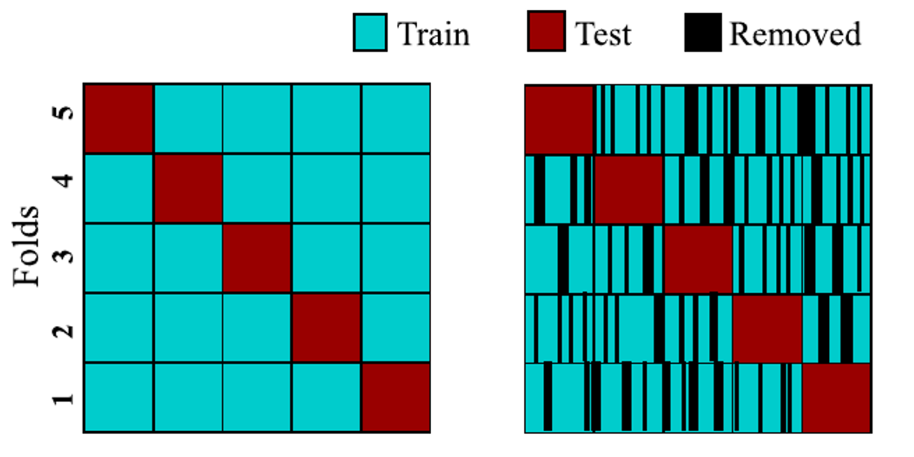
K-folds CV
Standard k-folds:
random shuffle
evenly spaced folds
possibly observations highly correlated with the test set are removed
Prequential (TS CV)
Since time series inherently deal with causality (past data has an effect on future data), the earliest and simplest time-series CV simply builds sets of increasing lengths (b). However:
the earliest fold is completely unrepresented. Earliest folds are trained on limited amount of data.
If hyperparameters are tuned, the selected ones are unlikely to work well on the full dataset
last folds are over-represented
To overcome these issues, sliding window approaches can be used, in which the test is done on a sliding window.
However, this approach is still not suited for data-driven models requiring high quantity of data.
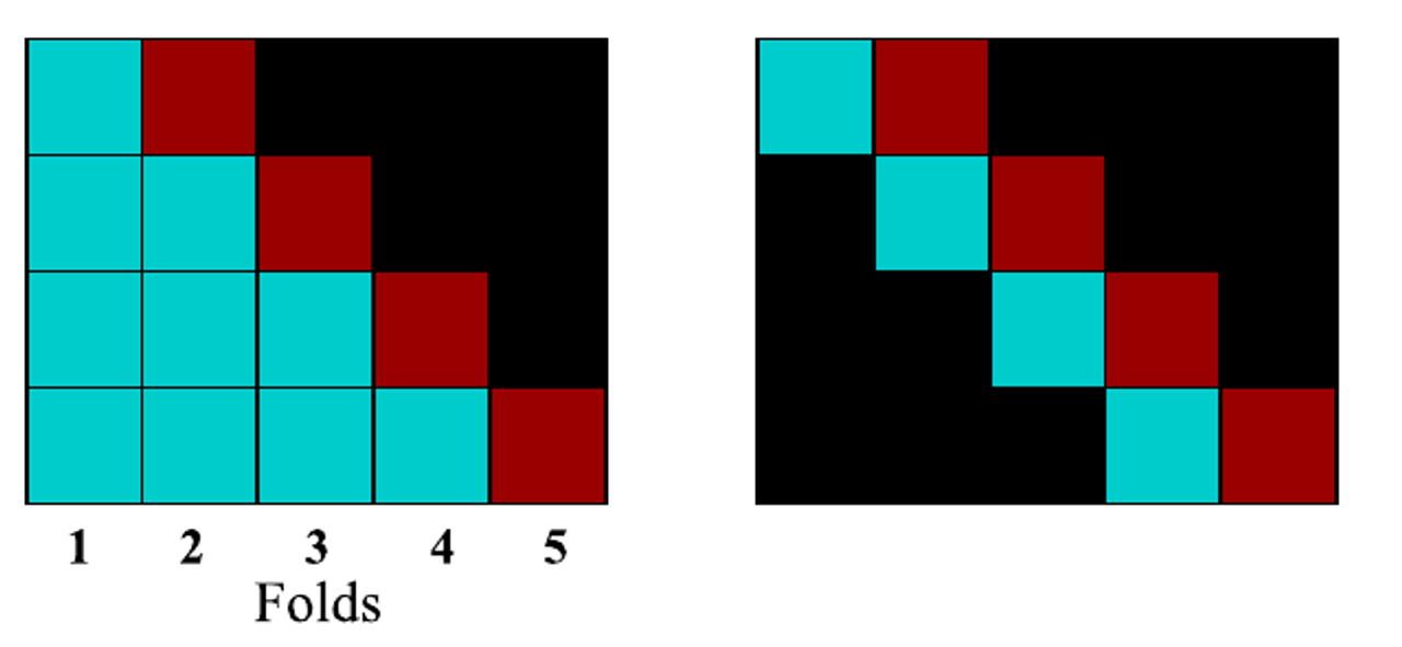
Left: classical TS-CV. RIght: sliding window approach
Purged approaches
The solution to this challenge is to realize that the
future can, in many cases, actually be used to forecast the
past, if we limit the data on each series appropriately. The
model and selected hyperparameters gain the benefit of a
full and robust training set, while each data point remains
aware of only its own past results. The key insight is to
purge or embargo some data between each fold, sufficient
to cover the longest forecasting interval
and any excess amount needed to prevent any short-
term trends appearing across multiple folds
- A.D.Lainder, R.D. Wolfinger, Forecasting with gradient boosted trees: augmentation, tuning, and cross-validation strategies Winning solution to the M5 Uncertainty competition, 2022
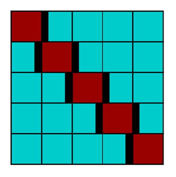
Data is not shuffled
Pairs of highly correlated data are removed
If data is using p past observations from the signal to predict n steps ahead, a good rule of thumb is to use p+n as embargo period
What happens if the best performing model out of the k folds is used as final forecaster?
Statistics for time-series model selection
Diebold-Mariano test
The Diebold-Mariano test is a statistical test used for comparing the accuracy of two sets of forecasts, at a given step ahead. The test compares the forecast errors for each set of forecasts and determines whether one set of forecasts is significantly more accurate than the other.
Defined d as the difference of the losses between two forecasters:
The Diebold-Mariano statistics is given by:
Where is the correlation at lag k of .
Under the assumption that there’s no difference between the two forecasts, we have that DM follows a Normal distribution:
The null hypothesis of no differences will be rejected if the DM statistics falls outside the range.
Small sample correction
For small sample sizes, DM test tends to reject the null hypothesis too often for small samples. A better test is the Harvey, Leybourne, and Newbold (HLN) test, which is based on the following:
The Nemenyi test is a post-hoc pairwise test, which is used to compare a set of m different models on a group of n independent experiments.
Usually performed after a Friedman’s test, which is a non-parametric analog of variance for a randomized block design. This test if there’s a difference in a set of n forecasters
a matrix whose elements are the ranks for experiment i and model j, is obtained.
The mean rank for each model is retrieved through column-wise averages of .
Friedman’s test for k algorithms on N datasets is used to see if there’s a difference between the k forecasters
The performance of two models is identified as significantly different by the Nemenyi test if the corresponding average ranks differ by
at least the critical difference:
where is the quantile α of the Studentized range statistic with N samples.
You can find an implementation of Nemenyi test for python in the scikit-posthocs library.