
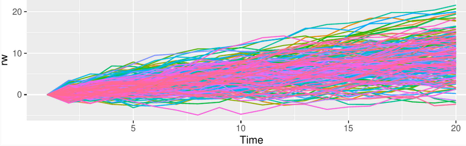
Consider the random process , also known as random walk with drift.
What’s the mean of the process at time t?
Is the process ergodic?
Can you make it stationary and ergodic by taking first differences?
Enforcing stationarity
We have seen that the random walk process
can be made mean-ergodic and stationary by taking the first order time derivative. Are there other methods to “regularize” a time series, so that we can better learn to predict it?
Transformations
Simple transformations are easier to explain and work well enough.
Transformations can have very large effect on PI.
log1p() can be useful for data with zeros.
Choosing logs is a simple way to force forecasts to be positive
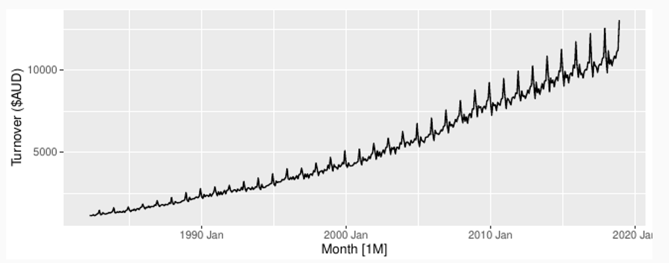
Original
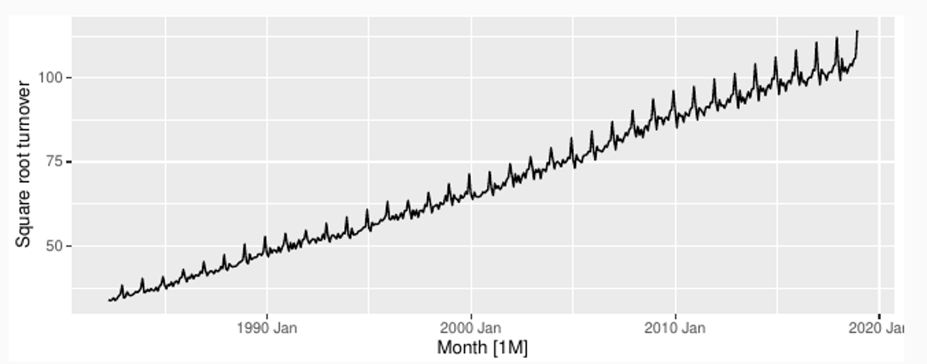
Square root
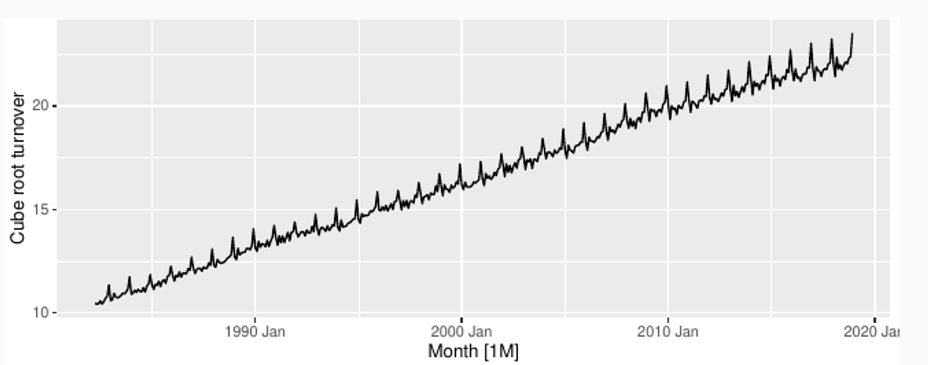
Cube root
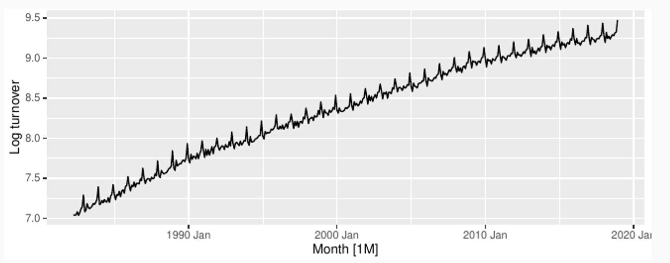
Log
In general, transformations can
be used to normalize the data and make it more suitable for modeling and analysis.
stabilize the variance of the data and reduce the impact of outliers.
improve the accuracy of statistical models and predictions by reducing the impact of non-normality in the data.
Box-Cox transform
For different choices of λ we get different transformations:
λ = 1: (No substantive transformation)
λ = 1/2 : (Square root plus linear transformation)
λ = 0: (Natural logarithm)
λ = −1: (Inverse plus 1)
Yeo–Johnson transform
Allows also for zero and negative values
λ = 1: Identity
General patterns - embeddings and sliding windows
General patterns - embeddings and sliding windows
A general pattern in univariate time series forecasting is to try to learn the time series dynamics from an embedding of past values. Time embedding is the fundamental techniques used by
exponential smoothing
state space models
AR, ARMA, ARIMAX models
stateless models (generic regressors)
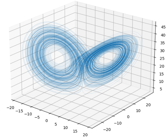
Time embedding for forecasting applications is mostly based on ideas from chaotic systems and system identification.
Takens theorem [1]: some chaotic systems can be deterministically determined by lags of the time series of their states. Furthermore, the system can be linearly embedded

[1] Huke, J. P. Embedding Nonlinear Dynamical Systems: A Guide to Takens’ Theorem
Taken’s theorem ensures we can predict the next values of x just considering the last 7 lagged values of x
Subspace system identification [2], one of the most used techniques to identify linear systems, creates a map between Hankel matrices of the inputs and outputs
[2] S. Joe Qin, An overview of subspace identification
Example: Lorenz system equations:
A linear state-space system can be described as a linear combination of states, inputs and noise
Subspace techniques identify the dynamic matrices starting from
Taken’s and Hankel matrices
A univariate time series , can be time-embedded in a -dimensional matrix using an embedding lag
If we get a Page or Taken’s matrix, when we call it an Hankel matrix.
The common idea behind these techniques is that the dynamics of an unknown system producing an observable time series can be learned from the data. Since, with no loss of generality, time series can be thought to be the output of a data generation process, we can try to apply these techniques to the forecasting task.
Moving averages and nonanticipativity
Besides considering the last lagged values of the time series, we can also apply transformations to the embedding matrix . For , taking the rows’ mean of computes the backward moving average of the signal.
Compare the centered (orange) and backward (green) 1-day moving average of the following signal. Which one can be used to forecast it? 
Centered (orange) and lagged (green) 2-days moving averages for a the power consumption of a Swiss DSO.
If the time series shows trends, a simple moving average can help making the series stationary, effectively un-correlating with its past and future lags →we can better estimate moments of distribution, and its joint CDF .
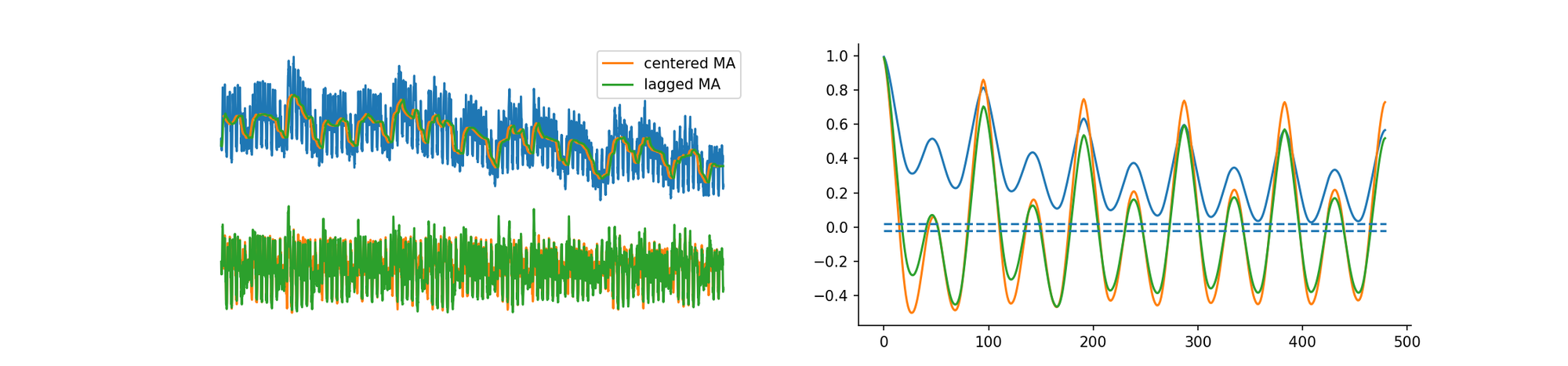
Effect of daily detrend on the ACF: the process becomes more stationary as lagged steps decorrelate
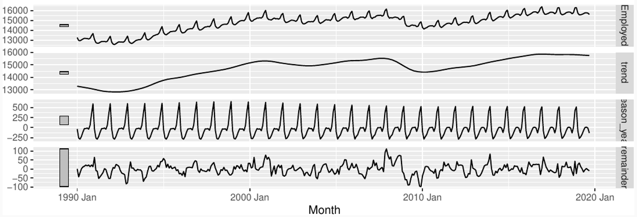
STL decompositions
STL decomposition is a popular method for decomposing a time series into its seasonal, trend, and remainder components. The acronym stands for "Seasonal and Trend decomposition using Loess," which refers to the technique used for estimating the components.
Seasonal time series can be decomposed as:
Since applying the log to both the side of the multiplicative decomposition form leads to
multiplicative decomposition → simply take the logarithm before applying the additive decomposition
We just need to estimate trend and seasonal components
The seasonal component is obtained by averaging over all seasons
Trend-cycle component is obtained by fitting a loess curve to the data
Pros:
Smoothness of trend-cycle also controlled by user.
Robust to outliers
Very versatile:
trend window controls loess bandwidth applied to de-seasonalised
values.
season window controls loess bandwidth applied to detrended
subseries
Anomaly detection in TS
Why?
Detecting outliers and anomalies and replacing or discarding them before fitting a forecasting model can positively increase the forecaster’s performance.
How?
Standard outlier filters can be adapted to time series data by applying them to sliding windows of the original signal
Sigma Filter and Hample filter
Sigma filter: mark as outlier if . Under normal distribution of the data, this filter corresponds to keep 99.7% of the observations
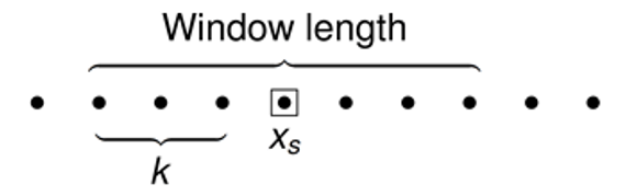
The Hample filter works by first calculating the mean and standard deviation of a sliding window of data points.
Centers the window of odd length at the current sample .
Computes the local median, , and standard deviation, , over the current window of data.
Compares the current sample with , where is the threshold value. If , the filter identifies the current sample, , as an outlier and replaces it with the median value, .
Boxplot Filter
The boxplot filter doesn’t assume a particular distribution. An observation is kept if:
where IQR is the interquartile range = . We can replace the sigma rule with the boxplot rule in the Hample filter to adapt it to time series data.
Do you think these filters can be combined with STL decomposition for seasonal time series? How?Spectral Residual Technique
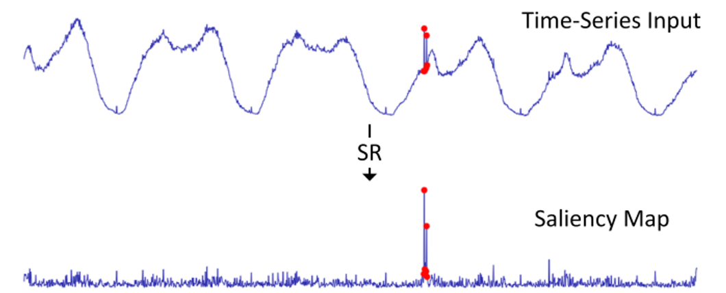
SR technique was proposed by researcher at Microsoft to spot anomalies in time series. It exploit information in the frequency domain by taking the Fourier transform of the time series, and consists of the following steps:
Take the log of the absolute value of the Fourier transform of the time series.
Smooth the log values using a rolling average.
Compute the spectral residuals by subtracting the smoothed log values from the log values.
Inverse Fourier transform the spectral residuals to obtain a saliency map or anomaly score
The anomaly score can then be used to identify regions of the time series that contain unusual activity. The SR technique has the advantage of being computationally efficient and easy to implement. Requires some parameter tuning to obtain good results.
Time-Series Anomaly Detection Service at Microsoft, H.Ren et al, 2019
Autoencoders
Autoencoders can be used to generate saliency maps and detect anomalies in TS.
Train an autoencoder on “good” data to predict sliding windows of the original signal, . The training is done minimizing reconstruction error
At inference time, run the autoencoder on new observed data, and use the reconstruction error as saliency map
Mark the observations as outliers if the reconstruction error is above a threshold
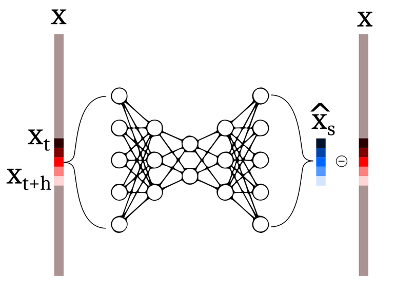
Schematics of a feed-forward autoencoder. The original sliding window is encoded in a vector with (usually) smaller dimensionality (latent representation), which is then used to reconstruct the original time series.
Forecast-based
We can combine ideas from the previous slides and define an anomaly detection strategy which is based on a forecasting model.
Given a forecasting model we can write:
If the future point can shows too extreme values of , we can mark it as an outlier.
Usually is chosen based on the assumed distribution of the error, for example normal gaussian. In this case we can use for example.
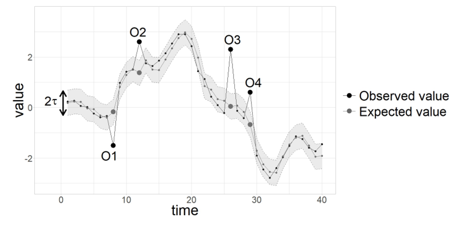
from: Blazquez-Garcia et al., A review on outlier/anomaly detection in time series data,2020 ACM
Data imputation in TS
Multivariate Imputation by Chained Equation
Multivariate Imputation by Chained Equation (MICE) is a popular method for imputing missing data in time series analysis.
The method involves using regression models to estimate the missing values of each variable in the time series, based on the other variables in the series. The process is repeated multiple times, with each iteration using the updated estimates of the missing values from the previous iterations to improve the accuracy of the imputations. MICE has the advantage of being able to handle missing data in multiple variables simultaneously, and can provide accurate imputations even when the missing data is non-random or correlated with other variables in the series.
Multivariate Imputation by Chained Equation (MICE) Method:
Create an imputation model for each variable with missing data.
Initialize the imputed values for each variable with missing data e.g. with mean
Iteratively update the imputed values for each variable with missing data, using the other variables in the time series as predictors.
Repeat the previous step until convergence or a maximum number of iterations is reached.
Use the imputed values to perform subsequent analyses.
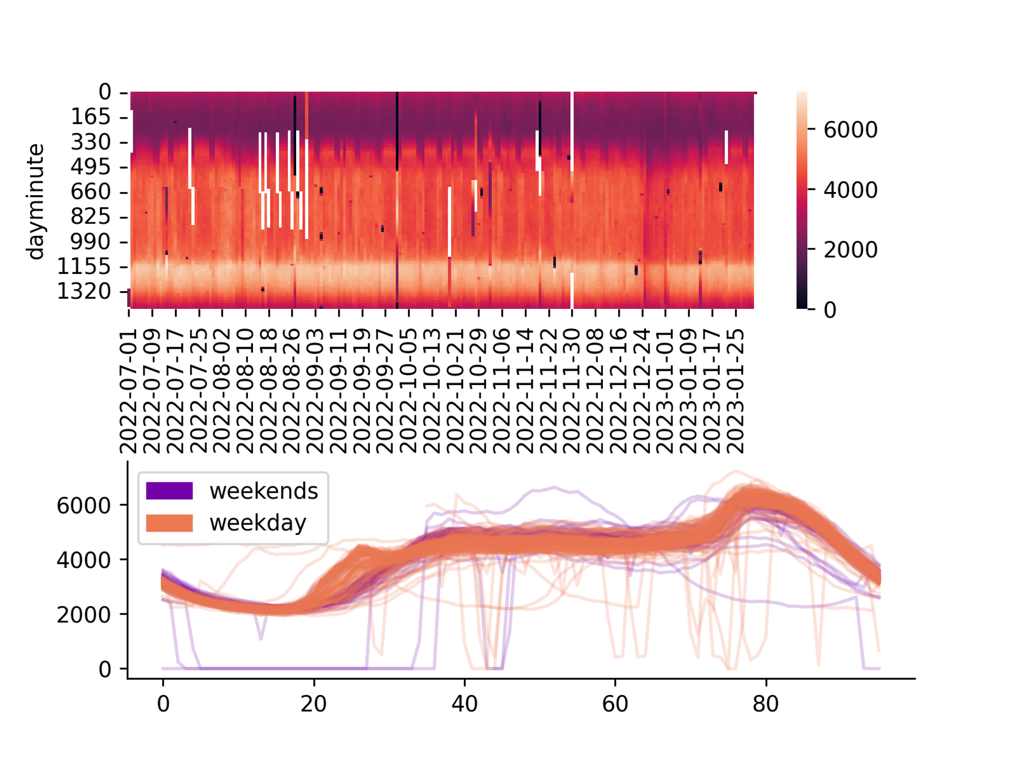
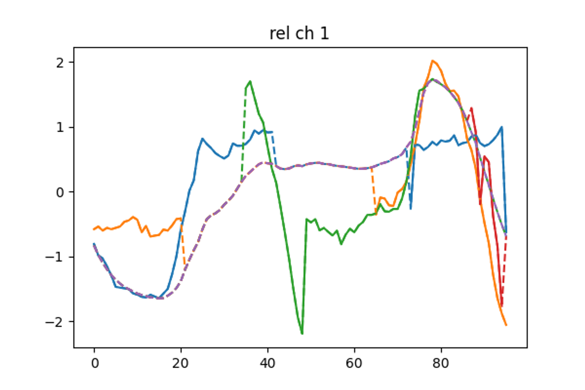
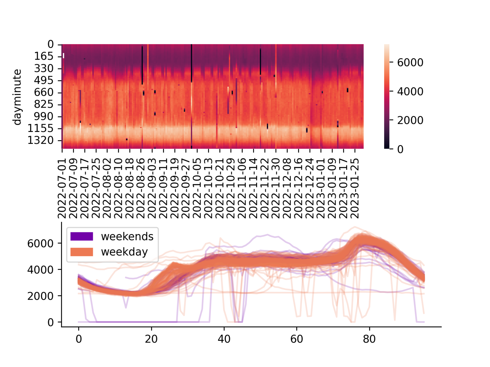
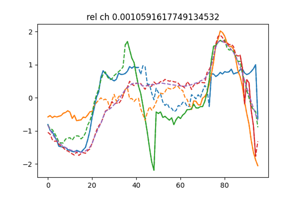
Expectation Maximization SVD
The EM-SVD algorithm is particularly indicated for seasonal data.
Normalize the daily embedded data by subtracting daily mean and dividing by the daily standard deviation
replace missing values with the mean values of the corresponding minute of the day
compute a truncated SVD decomposition of the matrix, using the first principal components
replace the missing data with the SVD approximation
repeat from point 3 until the algorithm converges. Convergence is reached when the mean change in missing data is below 1e-3.