


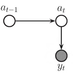
State space models, a brief introduction
State space models (sometimes known as latent variable models) are equivalent to HMMs
Assumptions:
markovian property
zero mean, iid Gaussian noise:
Additionally, we just consider stationary models, that is, parameters of are considered constant in time.
Applications:
Object tracking
Process modeling
Optimization
System identification and modeling
Forecasting
Exponential smoothing
ARMA / Box Jenkins
ARIMAX
All these applications have developed slightly different notations and consider slightly different terms and assumptions.
We will review them under a general framework / notation, from which all of them can be derived.
Linear, time invariant models
We will restrict the explanation to linear models, but all the explained properties hold also for non-linear models.
Moreover, we will assume that the parameters of the model are fixed in time.
Process form - Multiple source of errors
→ Kalman filter gain K →
Innovation form - Single source of error
All the tractation of exponential models for forecasting assumes an innovation form. We briefly review the Kalman filter theory which must be used to pass from process to innovation form.
Kalman filter
The Kalman filter is one of the most important and common estimation algorithms. It performs an exact Bayesian filtering for linear-Gaussian state space models. It can be used to:
estimate hidden (unknown) states based on a series of (noisy) measurements. Ex: GPS location and velocity = hidden states, differential time of the satellites' signals' arrival = measurements. Ex2: trajectory estimation for the Apollo program.
predict / forecast future system’s state based on past estimations. Ex: nowcasting
Example: tracking positions
Suppose we want to track the position of a robot in the woods, having just the readings of a unreliable GPS tracker.
We can write a useful state space model for the tracking using our knowledge on the laws of motion:
…write the balance equations in matrix form
…and obtain the stochastic formulation
Uncertainty propagation for linear-Gaussian variables
The zero-mean Gaussian distribution is completely determined by its covariance matrix
If the variable has a Gaussian distribution , so it has its linear transformation. You can view the linear operator as a superposition of two linear transformations: one on the mean value of , which can be treated as deterministic, and one on an associated zero-mean error distributed as :
Why is the covariance of the Gaussian rescaled in this way? From the definition of covariance:
Uncertainty propagation
In general, to improve the state estimation, it is useful to know if states are correlated. In this case, the robot could have higher velocities at particular positions (e.g. on a slope). Let’s assume the states have a Gaussian distribution where is the (symmetric) states’ covariance matrix.
How the state’s uncertainty spreads through time?
Deterministic step: shift
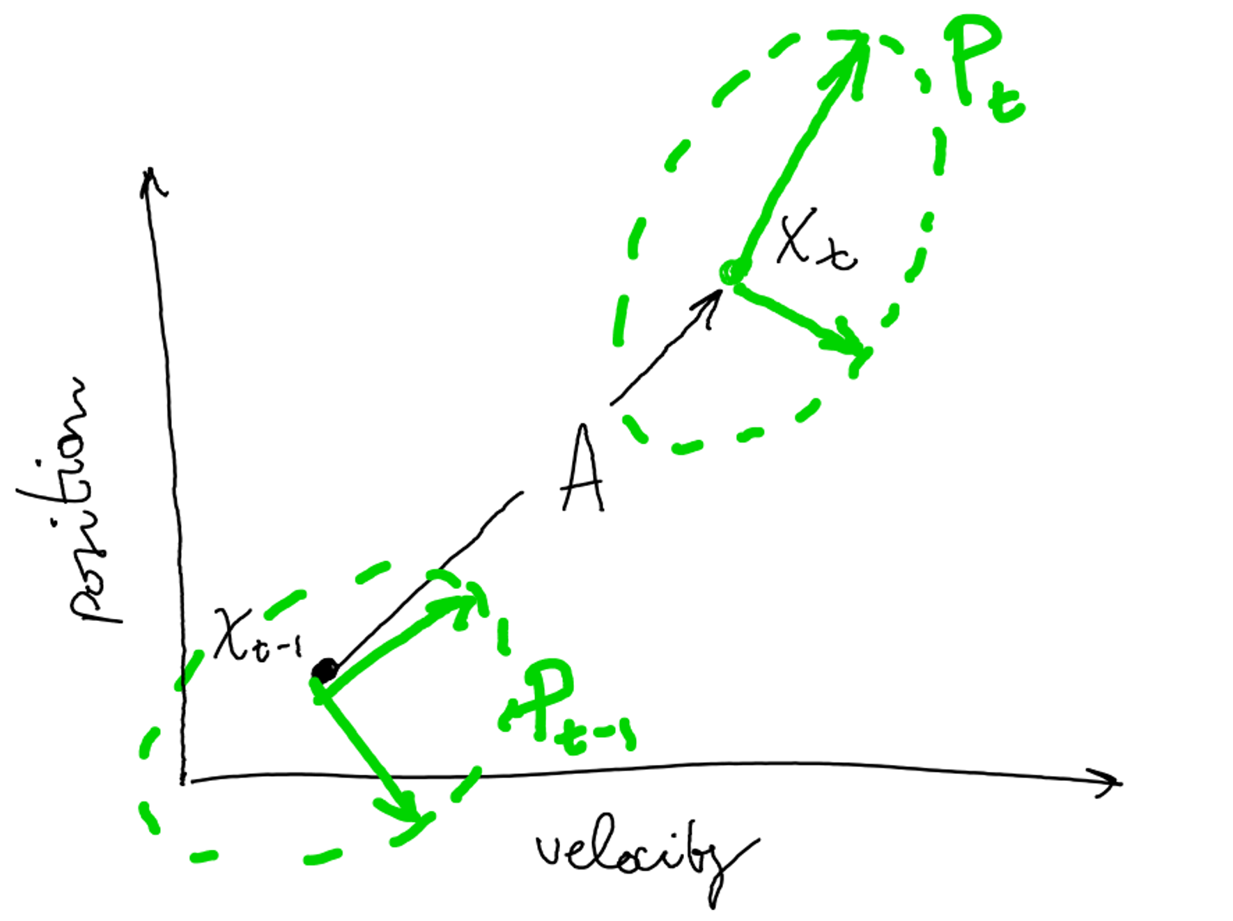
State uncertainty prediction for next step t, given the state covariance at time t-1
System noise: Gaussian blob→ still Gaussian
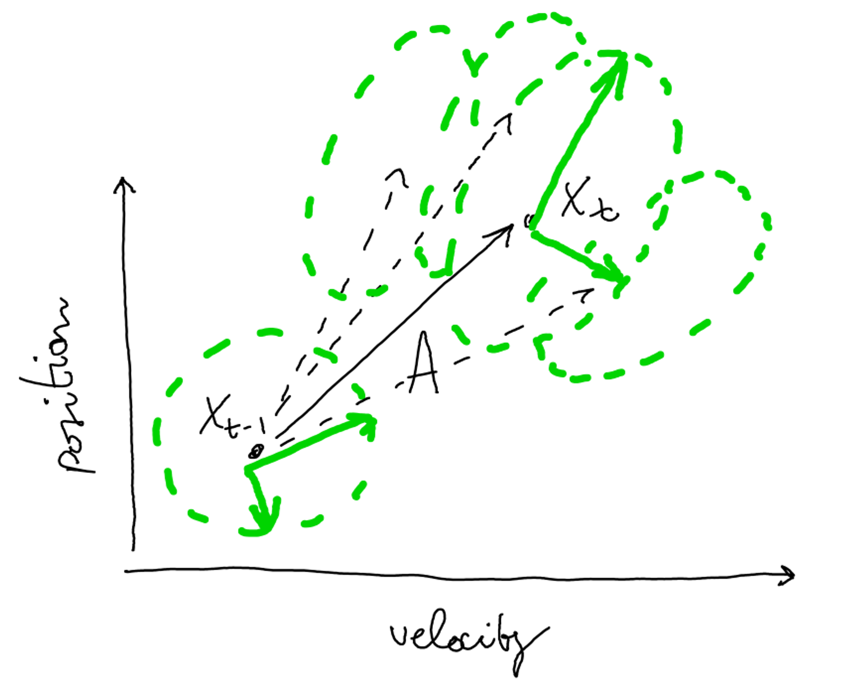
Additional uncertainty given by the system noise, affecting the next state’s prediction
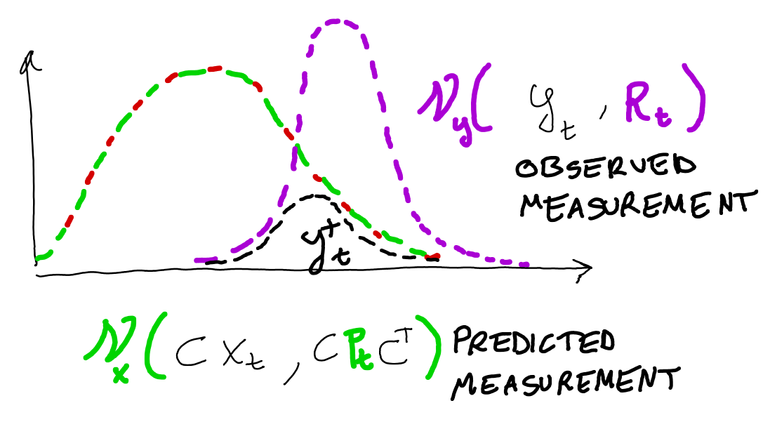
Exploit sensor’s observations:
predicted measurement
observed measurement
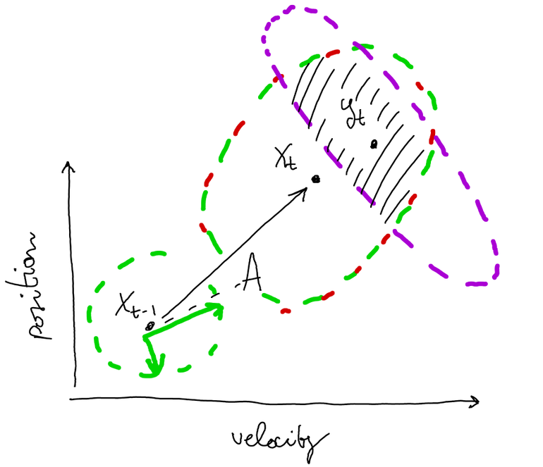
The uncertainty on the prediction can be reduced when we observe a new output from the GPS
Derivation of Kalman gain
The dashed space in the last picture shows the region where is most probable to find the state at time t, given the observations from the sensor. How does the predicted and observed measurements combine? Since we said that :
The multiplication of two univariate gaussians leads to:
We can then write
Interpretation: we are linearly correcting the measurement with the sensor’s values, with a weight proportional to the uncertainty on the predicted measure.
The covariance update can be written as:
Linear state space model estimation
 How can we estimate A, B, C, D, if we don’t observe state x?
Noise elimination
Since in the innovation form the noise enters both the equations at time t, we can eliminate one equation by substituting back in the first equation:
State elimination
We can now recursively find the state at the next step as an expression of previous inputs and observations:
start with
explicit next state as
repeat iteratively
By recursive substitution, we get:
We can see that at each step , the new state is a function of the initial state and a weighted sum of past inputs and observations .
If we now use the state at time as input to predict the new observation , we get:
This means that the forecasts of a state-space model in innovation form can be reformulated as a weighted sum of past observations and inputs. This form is also called the reduced form of the model.
This form show that ARIMA models can be formulated as SS models. Also exponential smoothing models can be formulated as SS, as we see in the following
Exponential smoothing
Trend component - simple exponential smoothing (T)
The simplest exponential smoothing just models the trend as a weighted sum between the last prediction and the last observation
By recursive substitution, this becomes:
…which represents a weighted moving average of all past observations with the weights decreasing exponentially, which smooths the observations
There are various methods that fall into the exponential smoothing family. Each has the property that forecasts are weighted combinations of past observations, with recent observations given relatively more weight than older observations. All share the name “exponential smoothing,” reflecting the fact that the weights decrease exponentially as the observations age.
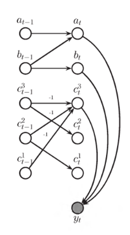
Equivalent representations
The component form gives the relations between the different model’s components. This is a procedural form, whose recursion gives the mean prediction. To pass from the component form to the state-space form, we must explicit the presence of measurement and process noise.
Component form
State Space form
Holt’s linear trend method (T)
Holt (1957) extended simple exponential smoothing to allow the forecasting of data with a trend.
Component form
State Space form
where denotes the estimation of the level, represents the change of level (that is, the slope), always estimated with an exponential smoothing
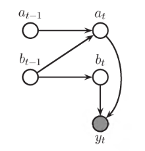
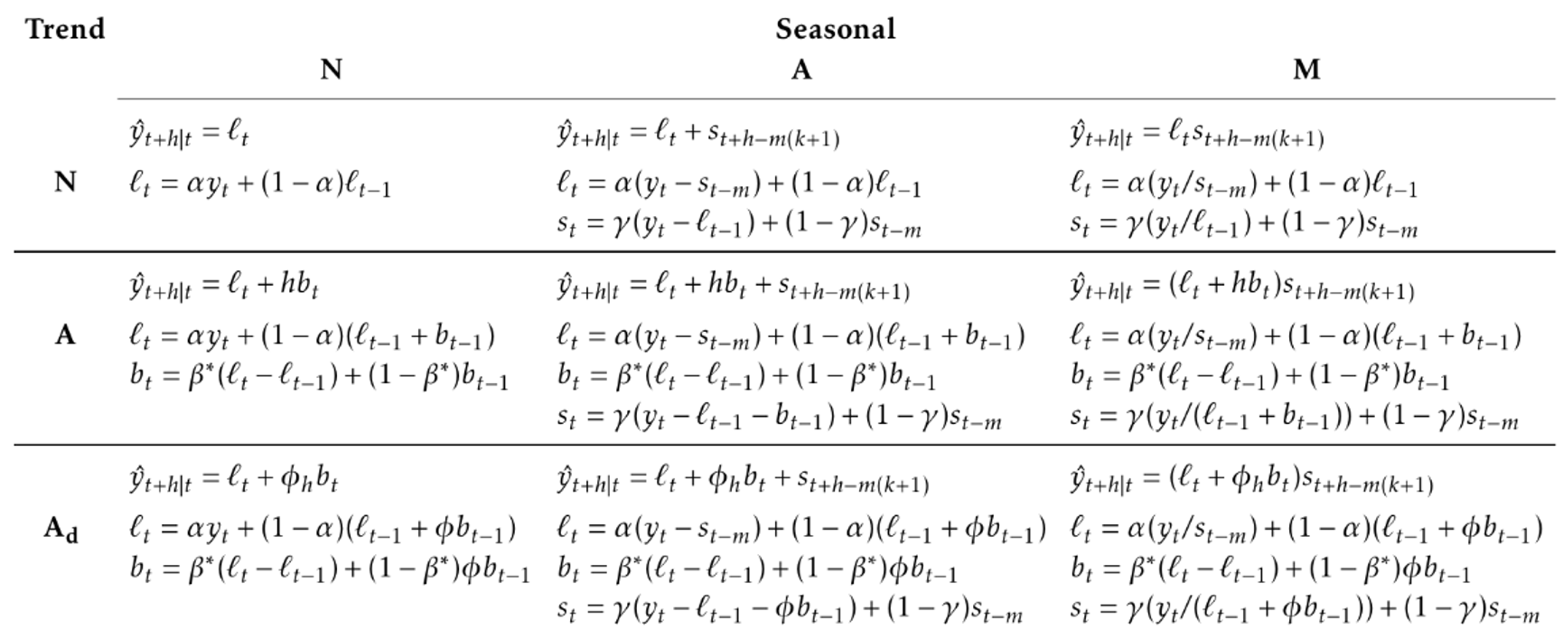
Holt’s Winters method
The Holt’s Winters method incorporates a single seasonality effect.
… and many more
Estimation
Unlike linear regression, no closed form → numerical optimization must be used.
Parameters are estimated maximising the likelihood.
For models with additive errors, equivalent to minimize the SSE
For models with multiplicative errors, not equivalent