Probabilistic forecasting

Probabilistic scores

Quantile loss

The quantile score is a linear expression of the prediction error ϵ=y−q^τ\epsilon = y-\hat{q}_{\tau}ϵ=y−q^​τ​﻿:

\begin{aligned}\rho_\tau(\epsilon)=&\epsilon\left(\tau-\mathbb{I}_{(\epsilon<0)}\right)\\ =& \begin{cases} \epsilon(\tau-1) \quad y<\hat{q}_{\tau} \\ \epsilon\tau \quad y>\hat{q}_{\tau} \end{cases}\end{aligned}

ALT

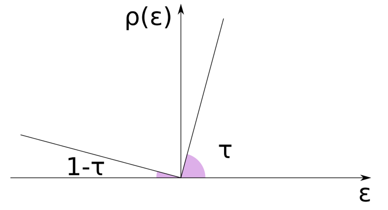
that, when minimized, is guaranteed to fit the τ\tauτ﻿-level quantile, regardless of the underlying distribution. We can see this minimizing the expected value of the quantile loss over the data distribution

We can split the expectation integral in two parts, under and above the predicted quantile:

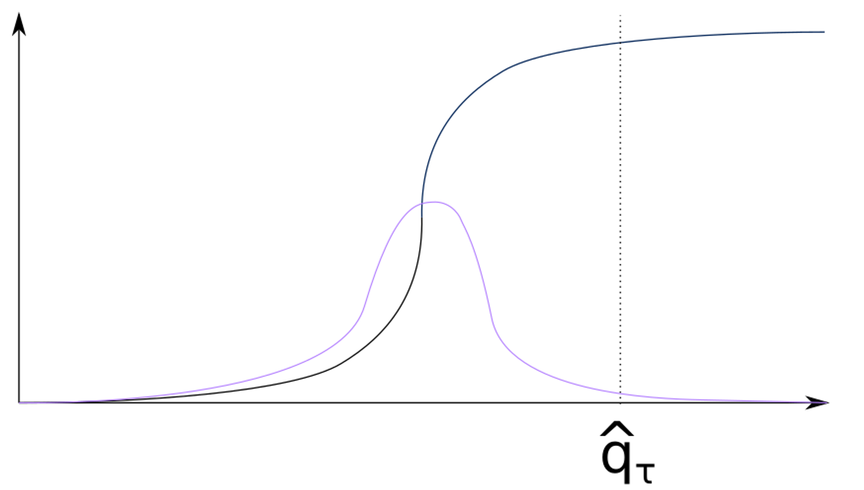
\underset{\hat{q}_\tau}{\arg \min }\left\{(\tau-1) \int_{-\infty}^{\hat{q}_\tau}(y-\hat{q}_\tau) d F_Y(y)+\tau \int_{\hat{q}_\tau}^{\infty}(y-\hat{q}_\tau) d F_Y(y)\right\}

and find the optimal value by deriving the expression by q^τ\hat{q}_{\tau}q^​τ​﻿ and setting it to 0:

(1-\tau) \int_{-\infty}^{\hat{q}_\tau} d F_Y(y)-\tau \int_{\hat{q}_\tau}^{\infty} d F_Y(y) = 0

The first integral is the definition of the CDF FY(q^τ)F_Y(\hat{q}_{\tau})FY​(q^​τ​)﻿, while the second is 1−FY(q^τ)1-F_Y(\hat{q}_{\tau})1−FY​(q^​τ​)﻿:

\begin{aligned}F_Y(\hat{q}_{\tau})-\tau &= 0\\ F_Y(\hat{q}_{\tau})&=\tau \end{aligned}

ALT

CRPS

The continuous rank probability score is defined as the quadratic distance between the forecasted CDF F^(z)\hat{F}(z)F^(z)﻿ and the empirical one. That is, CRPS computes how close the predicted quantiles are w.r.t. the data distribution:  

                                            Definition

\begin{aligned}\operatorname{CRPS}(f, y)&=\int_{-\infty}^{\infty} (\hat{F}(z)-\mathbb{I}\{y \leq z\})^2 \mathrm{d} z \end{aligned}

                                         Alternative formulation

\int_0^1 \rho_\tau\left(\hat{F}^{-1}(\tau), y\right) \mathrm{d} \tau

The CRPS is a proper scoring rule. Hence its minimum is obtained when F^(z)\hat{F}(z) F^(z)﻿ and the data distribution are equal

The first expression states that the CRPS can be computed by Montecarlo sampling from F^(z)\hat{F}(z)F^(z)﻿​

The second expression states that CRPS can be computed as the mean value of the quantile score over equispaced predicted quantiles F^−1\hat{F}^{-1}F^−1﻿​

Since CRSP depends on the scale of the signal, in order to compare it across different time series, it must be normalized with a benchmark forecaster:

CRSP_{norm} = \frac{CRSP_{ref} - CRSP}{CRSP_{ref}}

Reliability

A complementary measure of goodness of fit for a probabilistic prediction is reliability:

r_{\tau}(\hat{q}_\tau, y) = \frac{1}{N}\sum_{i=1}^{N} \mathbb{I}_{\{y<\hat{q}_\tau\}}

That is, reliability computes the average number of times the observations fall below a given quantile. 

CRPS and reliability can be easily computed. Here y∈Rnsy \in \mathbb{R}^{n_s}y∈Rns​﻿ is a vector of observed data and q∈Rnq×nsq \in \mathbb{R}^{n_q \times n_s}q∈Rnq​×ns​﻿ is a matrix whose rows contain the predicted tau-quantile: 

Python

Copy

def quantile_score(q, y, q_vect=np.arange(10)/10):
	qs = {}
	for tau, q_i in zip(q_vect, q):
	    err_tau = q_i - y
	    I = (err_tau > 0).astype(int)
	    qs[alpha] = np.mean((I - tau) * err_tau)

Python

Copy

def reliability(q, y, q_vect=np.arange(10)/10):
	res = {}
	for alpha, q_i in zip(q_vect, q):
	    res[alpha] = np.mean(y < q_i)

The CRPS is then the mean value of qs

Which is better

Consider the following 16 days dataset, for which we know the data generation process. We consider the following two predictions for the quantiles:

the empirical quantiles over the entire dataset (blue)

the empirical quantiles, conditional to each hour of the day (red)

If we generate the dataset again S times and evaluate the two strategies on the 17th day, which strategy will perform better in term of reliability and quantile scores? 

ALT

Distribution-agnostic probabilistic prediction methods

Naive bootstrap method

This method consists of:

train a model  MMM﻿ on Dtrain \mathcal{D}_{\text {train }} Dtrain ​﻿​

retrieve the error εM\varepsilon_MεM​﻿ on the training set

superimpose quantiles of εM\varepsilon_MεM​﻿ to the predictions, so that the final confidence interval is [y^t+1−q1−τ(ε),y^t+1+qτ(ε)]\left[\hat{y}_{t+1}-q_{1-\tau}(\varepsilon), \hat{y}_{t+1}+q_{\tau}(\varepsilon)\right][y^​t+1​−q1−τ​(ε),y^​t+1​+qτ​(ε)]﻿​

​

fast, distribution and model agnostic

​

Using the training set for retrieving the empirical distribution makes the prediction intervals over-confident

Quantile regression

We have seen that the minimizer of the quantile loss is the empirical tau-quantile, regardless of the underlying distribution →  quantile regression consists of training a regressor to directly minimize the quantile loss ρτ(ϵ)\rho_{\tau}(\epsilon)ρτ​(ϵ)﻿.  

​

agnostic to the data distribution

can be directly minimized by generic regressors (LightGBM, kNN, NNs)

independent models for different steps ahead

​

We need to train separate models for separate steps-ahead AND quantile levels

Since quantiles are independently trained, we can experience quantile crossing

The M5 competition winner for the probabilistic track used a set of LightGBM, minimizing the quantile loss.  

Conformal predictions

Conformal prediction is based on the idea of constructing a set of hypothesis tests to determine whether a new observation is consistent with the previously observed data. The test results are then used to construct a prediction interval, which is guaranteed to contain the true value with a certain probability. 

Conformal prediction doesn’t require IID assumption but requires exchangeability: any permutation of the dataset observations is equiprobable. However, the time steps within a time-series are inherently non-exchangeable due to temporal dependencies. 

Given a dataset D={(x(i),y(i))}i=1l\mathcal{D}=\left\{\left(\mathbf{x}^{(i)}, y^{(i)}\right)\right\}_{i=1}^lD={(x(i),y(i))}i=1l​﻿, CP generates prediction intervals such that: 

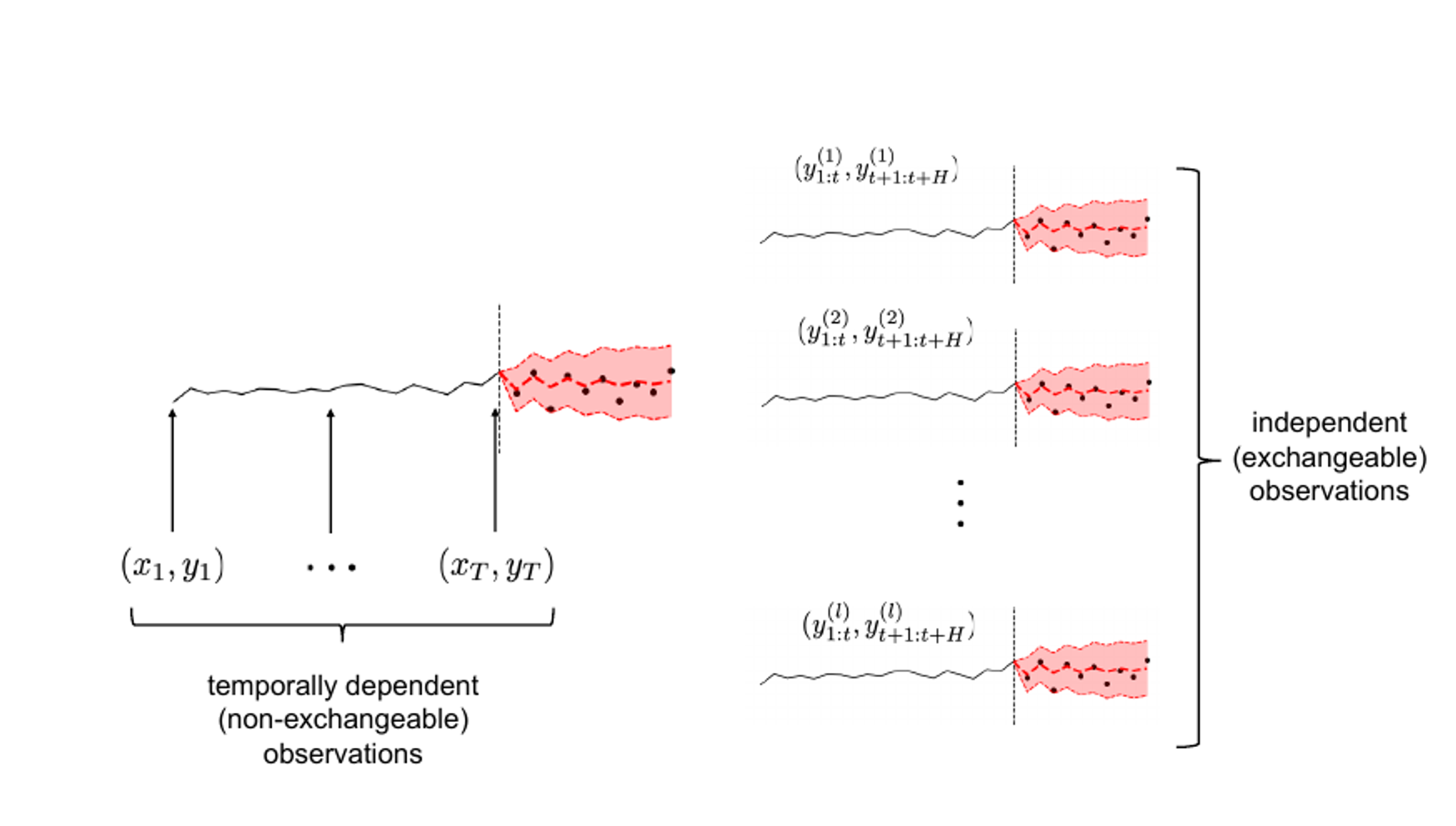
\mathbb{P}\left[y_{t+1} \in \Gamma^\alpha\left(\mathbf{x}_{t+1}\right) \mid \mathcal{D}\right] \geq 1-\alpha

ALT

Left: time series can’t be considered exchangeable. Right: exchangeability can be obtained considering several instances of multiple step-ahead forecasting (=embeddings). 

ALT

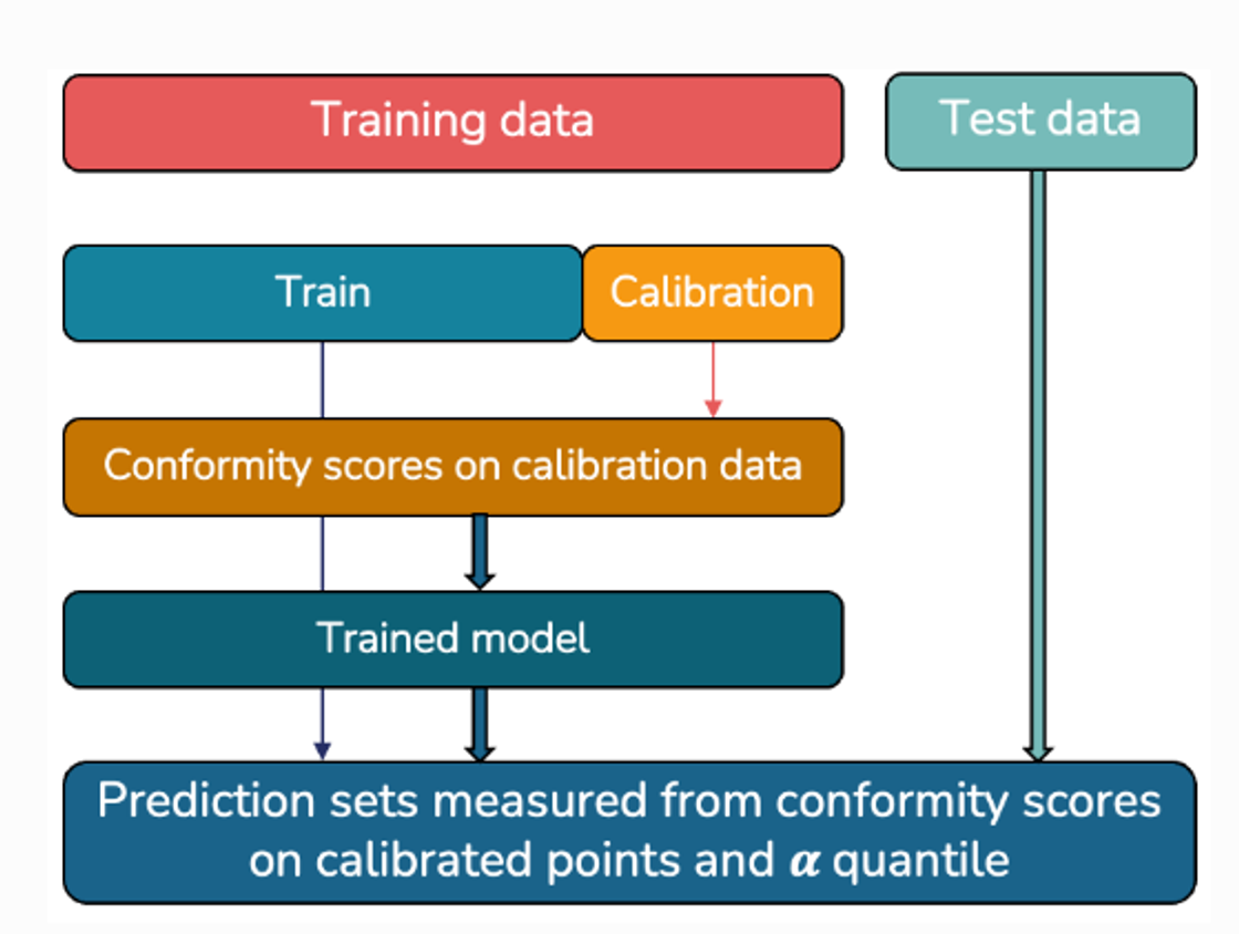
CP theory is pretty involved, but the steps of the basic method can be summarized as:

Split the dataset in training and calibration D=Dtrain ∪Dcal \mathcal{D}=\mathcal{D}_{\text {train }} \cup \mathcal{D}_{\text {cal }}D=Dtrain ​∪Dcal ​﻿​

Train a forecasting model MMM﻿ on Dtrain \mathcal{D}_{\text {train }} Dtrain ​﻿​

Use the calibration set Dcal\mathcal{D}_{\text {cal}}  Dcal​﻿ to obtain a non-conformity score: a measure of how much new predictions differ from observed ones. Usually the non-conformity score is the absolute value of the prediction error.

 Compute prediction intervals as Γα(xt+1)=[y^t+1−ε^,y^t+1+ε^]\Gamma^\alpha\left(\mathbf{x}_{t+1}\right)=\left[\hat{y}_{t+1}-\hat{\varepsilon}, \hat{y}_{t+1}+\hat{\varepsilon}\right]Γα(xt+1​)=[y^​t+1​−ε^,y^​t+1​+ε^]﻿  where y^t+1=M(xt+1)\hat{y}_{t+1} = M(\mathbf{x}_{t+1})y^​t+1​=M(xt+1​)﻿ and ε^\hat{\varepsilon} ε^﻿ is the 1−α1-\alpha1−α﻿ quantile of the prediction error on Dcal\mathcal{D}_{\text {cal}}  Dcal​﻿, ordered with the conformity score.

ALT

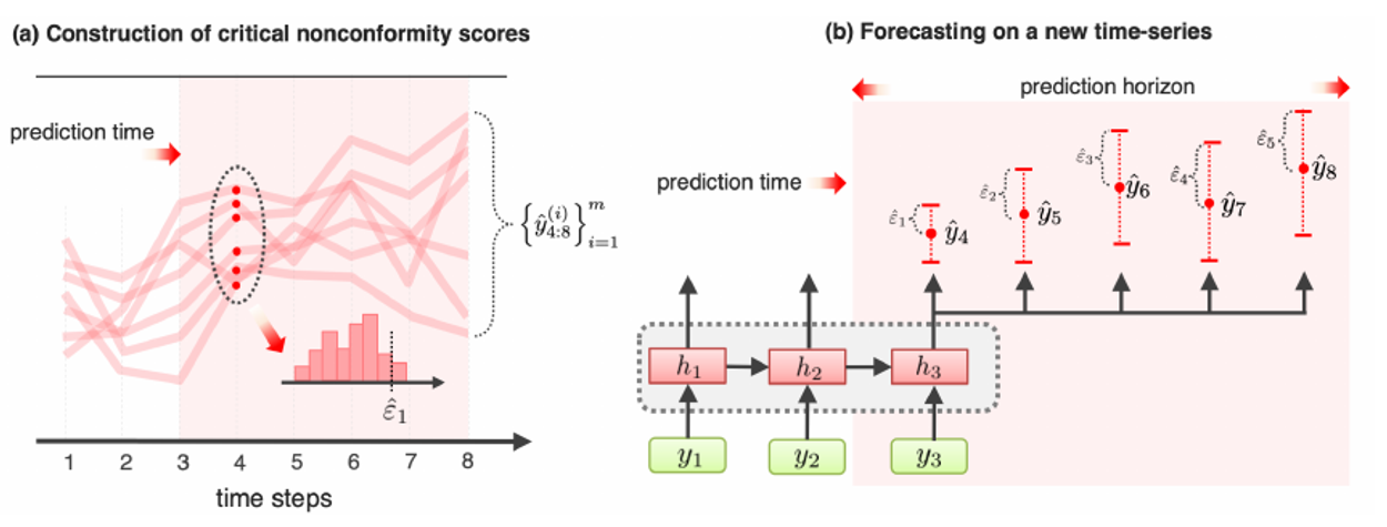
CP intervals for multi step-ahead predictions: each step ahead has its own error distribution 

ALT

When the non-conformity score is the prediction error, this method corresponds to the naive bootstrap method.

The only difference is that for multi-step-ahead forecasts, CP applies a Bonferroni correction: instead of taking the τ\tauτ﻿ quantile, we take the τ±(1−τ)/ns\tau \pm  (1-\tau)/n_{s}τ±(1−τ)/ns​﻿ quantile, where the sign depends on whether we are computing a quantile lower (-) than 0.5 or higher (+).

Cross-conformal predictors

In the base form, CP sacrifices part of the dataset for calibration. To increase data efficiency, CP can be combined with CV using the following scheme:

A CV scheme is applied:

For each split, confidence intervals are generated from perturbed models

ALT

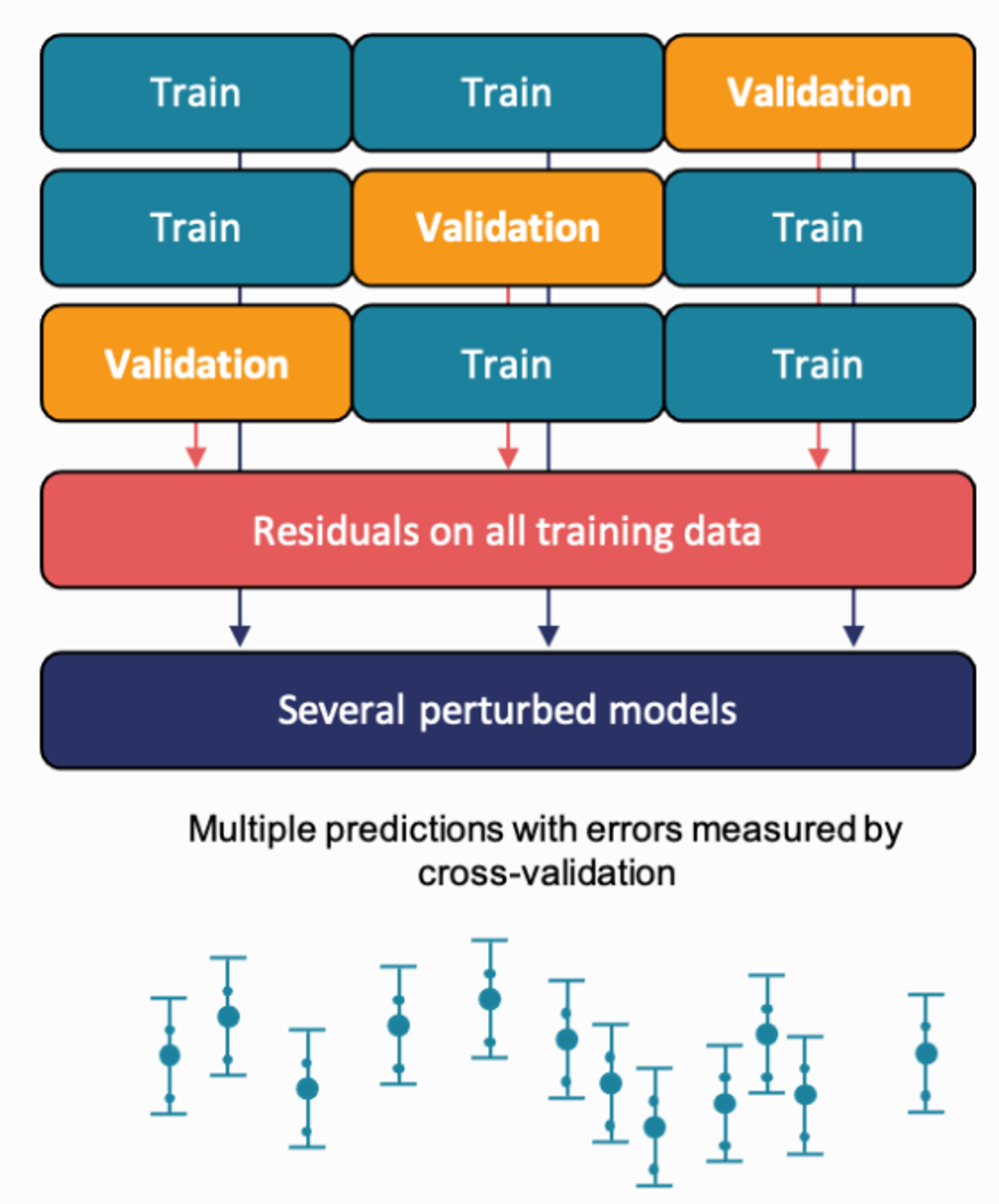
Each fold is composed of the following steps:

A model MMM﻿ is trained on part of the training data

conformity scores are obtained on the rest of the training data

The test data 

ALT

Variants of CP, as conformalized quantile regression (CQR), use the quantile loss to better calibrate the prediction intervals on heteroscedastic data.  

​

non-parametric, distribution-agnostic 

can produce consistent probabilistic distributions for multiple steps ahead 

has been applied in a wide range of domains, including finance, medicine, and meteorology, among others.

different plug-and-play libraries, like MAPIE, provide CP intervals for scikit-learn compatible models 

​

in the base form, it doesn’t produce conditional intervals 

Advanced methods

Estimation of multivariate PDFs using copulas

Estimating time-varying and high-dimensional covariance matrices often limits existing methods to handling at most a few hundred dimensions or
requires making strong assumptions on the dependence between series

ALT

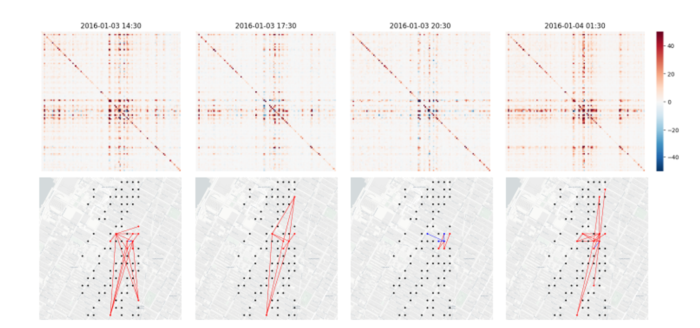
Time-varying covariance matrices for taxi traffic time series for 1214 locations in New-York at 4 different hours of a Sunday

ALT

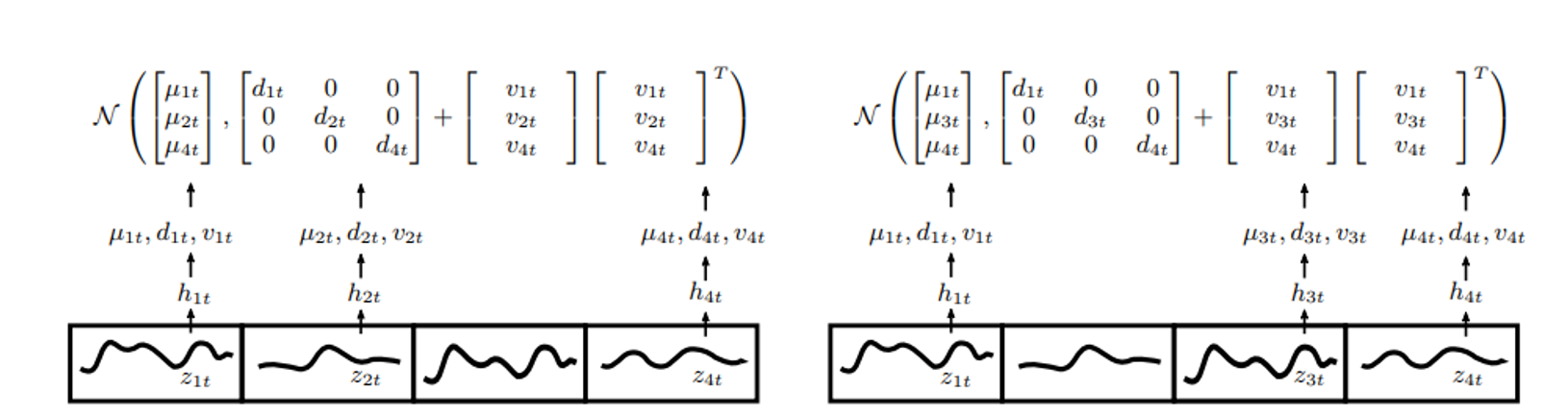
Gaussian copula process output model to handle non-Gaussian marginal distributions

low-rank covariance structure to reduce the computational complexity 

ALT

From “Salinas D. et al., High-Dimensional Multivariate Forecasting with Low-Rank Gaussian Copula Processes”, NeurIPS 2019

ALT

Scenario generation

Forecasting techniques usually generate different PDFs for different timesteps. 

They do not directly output the whole joint distribution    Fx1,…xN(b1,…,bN)=P(x1(ω)≤b1,…,xN(ω)≤bN)

F_{x_1, \dots x_N}\left(b_1, \dots, b_N\right)=\mathrm{P}\left(x_1(\omega) \leq b_1,\dots,x_N(\omega) \leq b_N\right)Fx1​,…xN​​(b1​,…,bN​)=P(x1​(ω)≤b1​,…,xN​(ω)≤bN​)﻿ from which we could derive all the properties of the stochastic process. 

As for the hierarchical reconciliation technique, usually, an ex-post method is used to produce scenarios.

ALT

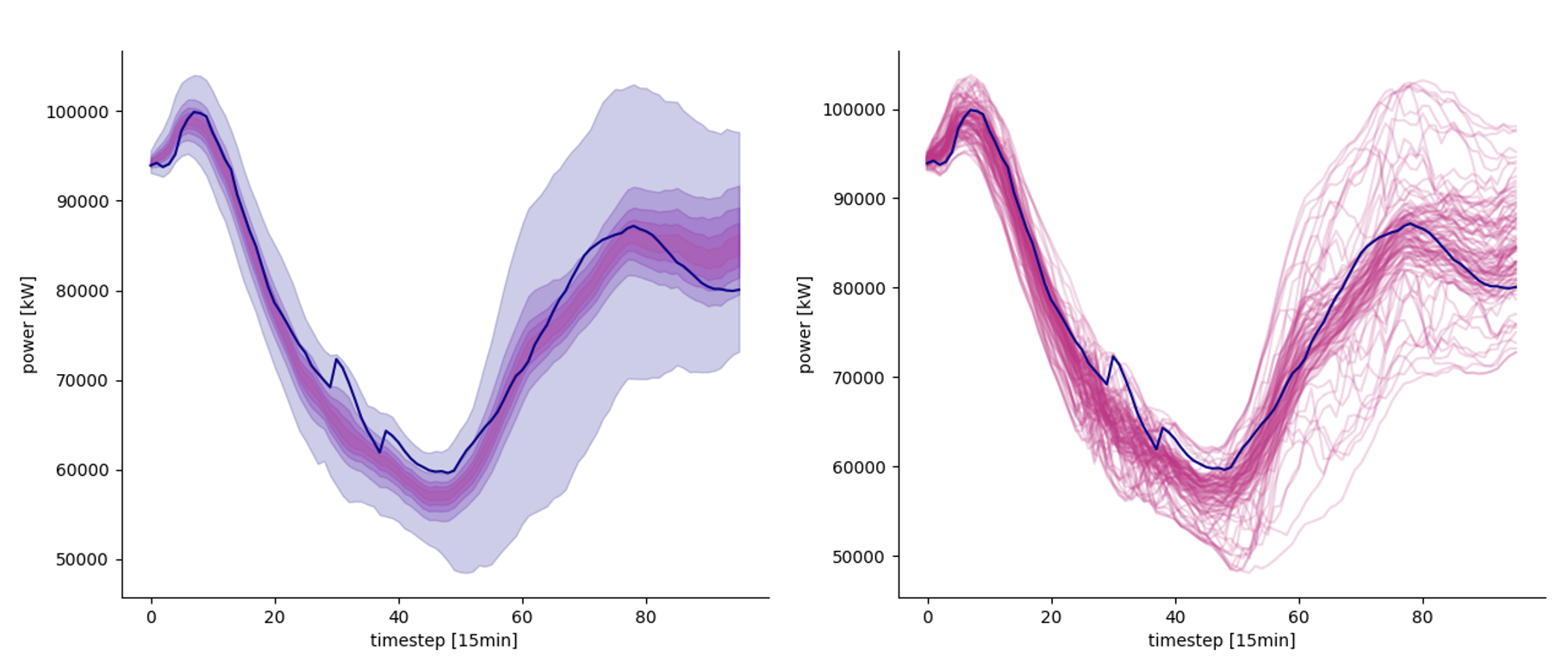
Left: predicted quantiles. Right: 100 different scenarios

ALT

Linking PDFs through correlation structure

Recall that we can generate new samples from a univariate distribution, known its analytical or empirical CDF Fx(b)F_x(b) Fx​(b)﻿, by means of the inverse probability transform:

Fx(b)=P(x(ω)≤b)F_x\left(b\right)=\mathrm{P}\left(x(\omega) \leq b\right)Fx​(b)=P(x(ω)≤b)﻿​

Fx(x)=UF_x(x) = UFx​(x)=U﻿​

xnew=F−1(unew)x_{new} = F^{-1}(u_{new})xnew​=F−1(unew​)﻿​

…simply means that querying the CDF on the y axis will sample new observations xnewx_{new}xnew​﻿ whose density function is the original PDF

ALT

How can we sample from a multivariate distribution by independently query the marginals ?

if a method exists, it must produce consistent marginals P(x1∣x2…xN)∼Fx1P(x_1\vert x_2\dots x_N) \sim F_{x_1} P(x1​∣x2​…xN​)∼Fx1​​﻿ → we can use multivariate uniform distribution with a dependence structure

Copulas C:[0,1]N→[0,1]C:[0,1]^N \rightarrow[0,1]C:[0,1]N→[0,1]﻿ are multivariate CDFs with uniform marginals. 

C\left(u_1, \ldots, u_N\right)=P\left(U_1 \leq u_1, \ldots, U_N \leq u_N\right)

Sklar’s theorem states that any joint CDF can be expressed starting from its marginals, linked by a copula

F\left(z_1, \ldots, z_N\right)=C\left(F_1\left(z_1\right), \ldots, F_N\left(z_N\right)\right)

For a lot of real multivariate processes, the covariance structure can be modeled using a multivariate Gaussian N(0,Σ)\mathcal{N}(0, \Sigma)N(0,Σ)﻿​

estimate Σ\Sigma Σ﻿ from the observed data

produce multivariate Gaussian samples, :  [zi]i=1N∼N(0,Σ)[z_i]_{i=1}^N \sim \mathcal{N}(0, \Sigma)[zi​]i=1N​∼N(0,Σ)﻿​

use the inverse probability transform to obtain uniform random variables in the [0, 1] range through the normal ECDF [ui]i=1N∼Φ(N(0,Σ))[u_i]_{i=1}^N \sim  \Phi(\mathcal{N}(0, \Sigma)) [ui​]i=1N​∼Φ(N(0,Σ))﻿ 

query each marginal ECDF independently, but using the correlated uniform samples xi=Fi−1(ui)x_i = F^{-1}_i(u_i)xi​=Fi−1​(ui​)﻿​

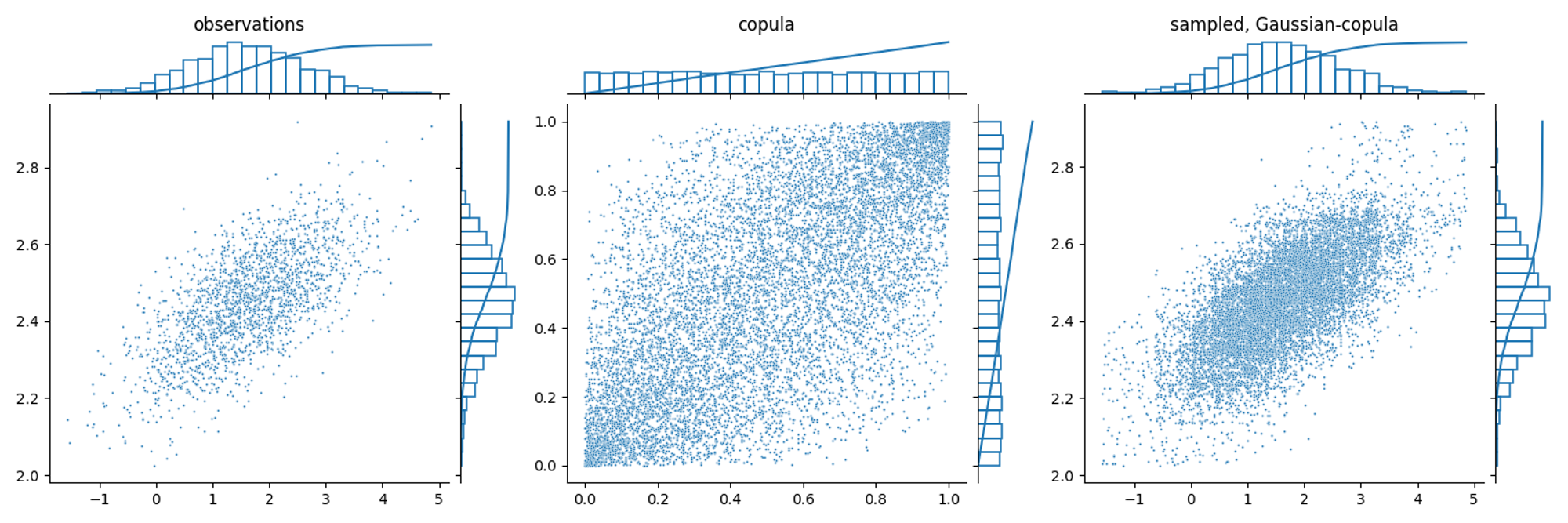
Unimodal example

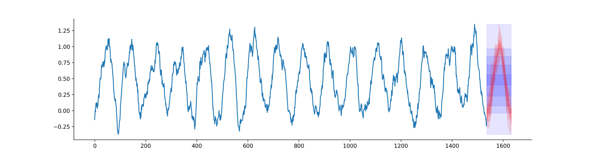
Imagine that we want to model the correlation between the first two steps ahead forecasts. We can use this method to create a generative model 

            1: Estimate Σ\SigmaΣ﻿ from observation 

             2-3: [zi]i=1N∼Φ(N(0,Σ))[z_i]_{i=1}^N \sim \Phi(\mathcal{N}(0, \Sigma))[zi​]i=1N​∼Φ(N(0,Σ))﻿​

                     4: xi=Fi−1(ui)x_i = F^{-1}_i(u_i)xi​=Fi−1​(ui​)﻿​

ALT

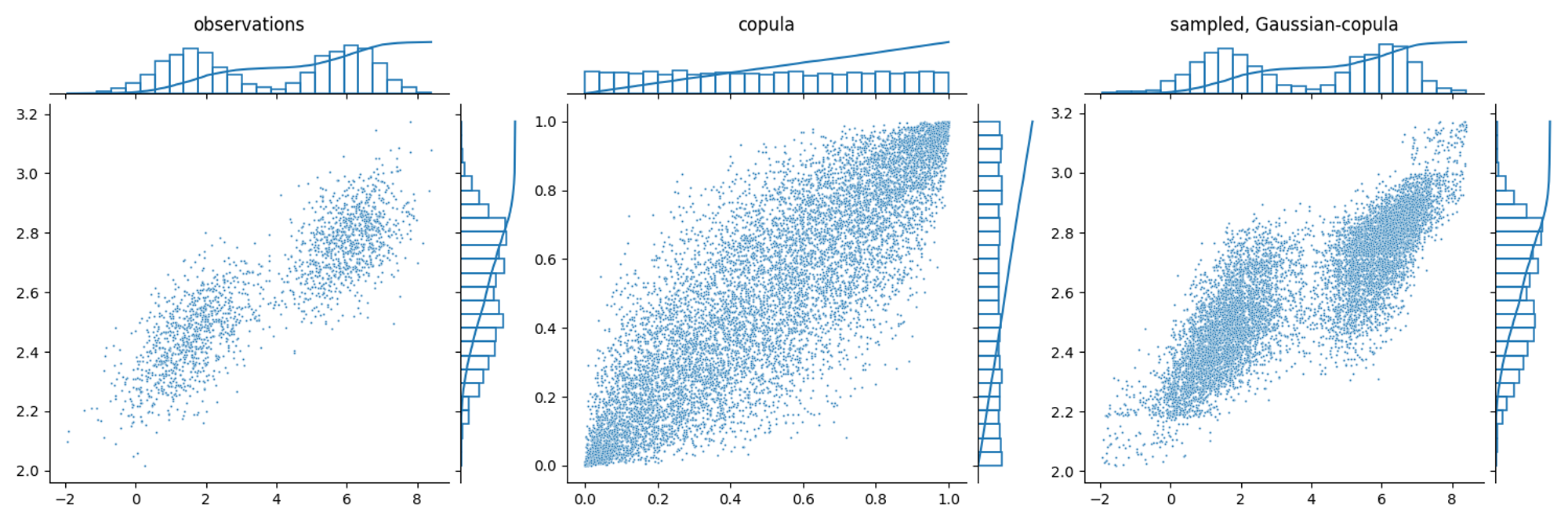
Multimodal example

Gaussian correlation can also be applied to non-gaussian correlation structure or bimodal marginal distribution. However, in this case the generated samples won’t perfectly resemble the observed distributions. 

ALT

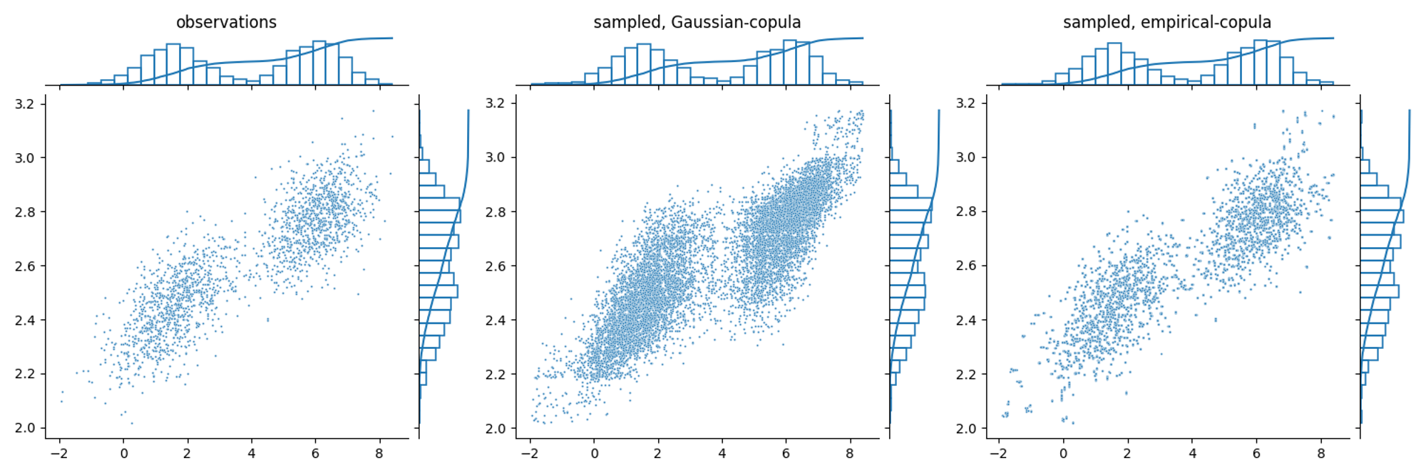
Empirical copula coupling example

Another method is to directly use the observed copula structure to generate new samples.

ALT

Stochastic trees

Forecast scenarios can be used directly in robust optimization. Usually, when the dynamics of the decision process is important, scenarios are reduced into a stochastic tree representation of the uncertainty.

ALT

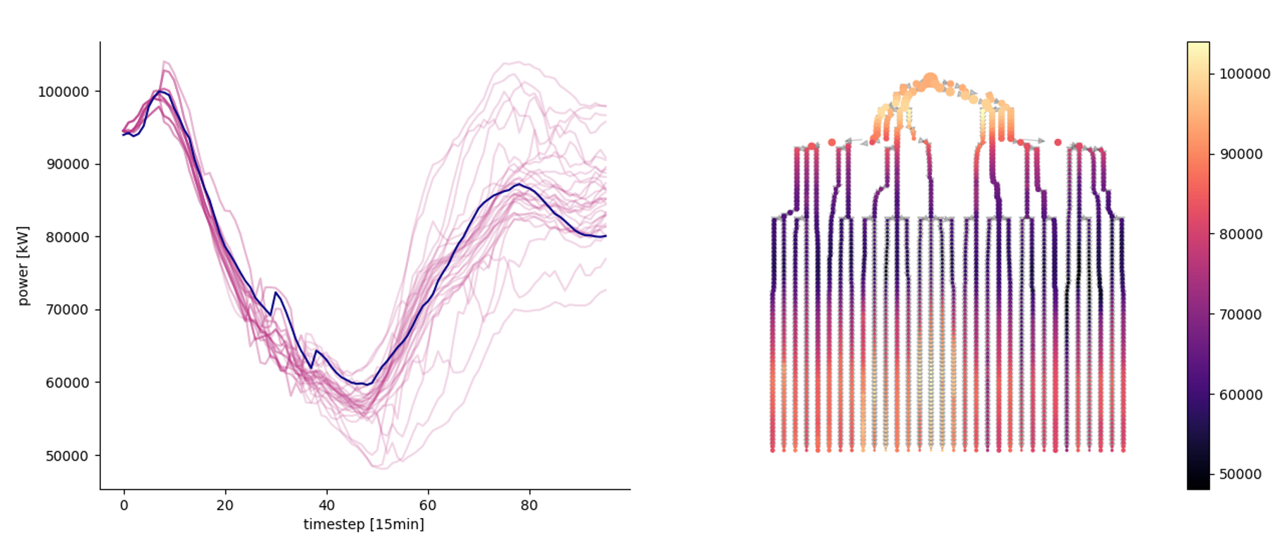
Left: a stochastic scenario tree obtained from the scenarios. Right: graph representation of the tree

ALT

Backward/Forward algorithm

The problem of reducing N scenarios to a tree is in general a hard problem. It is equivalent to an optimal transport problem, where we want minimize the distance of two multivariate distributions: the original one and the tree-encoded one. 

Usually,  some heuristics are applied. 

The forward/backward methods consist of recursively pruning and merging scenarios based on their importance. 

Backward method:

starting from T, aggregate closer scenarios based on a threshold distance

merged scenarios increase their weight = holding probability

the process is repeated back to t=0

Forward method

starting from t=0, aggregate closer scenarios based on a threshold distance

merged scenarios increase their weight = holding probability

the process is repeated back to t=T

ALT

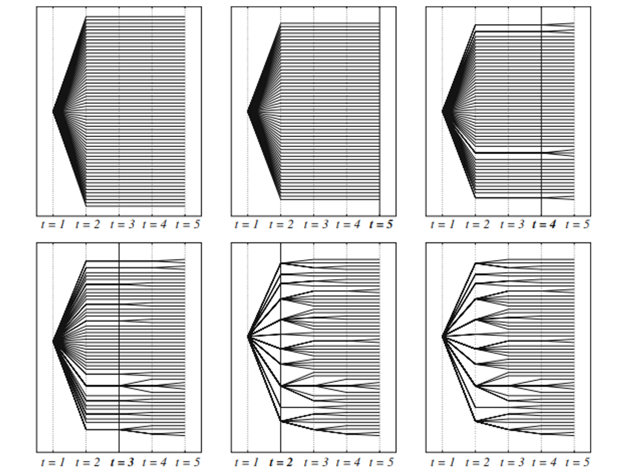
backward selection method

ALT

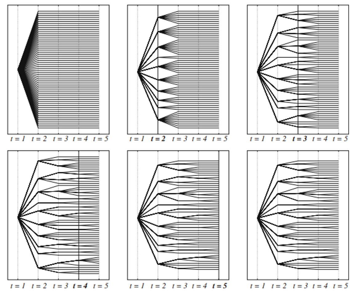
forward selection method

ALT

Neural gas & Direct loss minimization

The backward/forward heuristics do not allow for a fixed tree structure. Keeping a fixed tree structure is important if we want to pass it to a learning method, such as RL. 

Two methods that keep a fixed structure are:

Neural Gas method: this is based on self-organizing maps. It’s an iterative method where “neurons” (nodes of the tree) are iteratively shifted based on their weighted distance from the data points. Convergence must be enforced by a shrinking learning rate.

Direct minimization of the original data distribution and the tree-encoded one. This can be achieved by gradient descent and auto-differentiation. Neither this method is guaranteed to converge to the global optimum, but it usually achieves good results. 

ALT

Neural gas for scenario tree reduction

ALT

Direct differentiation of the reconstruction loss

ALT