Hierarchical forecasting

…there is a lot of potential in this particular area of forecasting and that developing new hierarchical forecasting methods, capable of reconciling forecasts so that the forecast error is minimized, not only on average but separately at each aggregation level, could provide substantial accuracy improvements.

Makridakis - “M5 accuracy competition: Results, findings, and conclusions”
2022, International Journal of Forecasting

Why consistent forecasts? Some examples

In many occasions, more than one signal must be forecasted. If we know that the signals are subject to an algebraic relation, we would like their forecast to respect it as well. Why?

Sales at different aggregation levels

Using consistent forecasts for sales at different aggregation levels is important in logistic planning. Inconsistent forecasts leads to unnecessary stock accumulations or lack of availability. 

Water distribution network

Valves and pumps must be jointly controlled to keep water pressure within the network, as a function of the predicted demand. If the forecasted demand of the pipes drawing from the same vassel doesn’t sum up, our control actions will lead to a pressure change.

Distributed demand side management

Consider a district with a residential battery trying to perform peak shaving, and residential batteries trying to maximize self consumption. If forecasts are not consistent, the battery at the feeder will try to compensate actions of the privately-owned batteries, leading to an economic loss.

PV power production
Consider a region with a high penetration of PV power plants. Considering independent CDFs for the power produced by the PV power plants will result in an overall narrow CDF, since errors will tend to compensate for each other. In practice, the predictions of PV power plants of the same region have highly correlated errors, since all heavily depend on the same irradiance and temperature forecasts. Probabilistic reconciliation can produce more accurate CDF of the total produced power.

Another reason to work on reconciliation techniques is that, if the number of TS to forecast is high, it is hard to directly produce a set of consistent by design forecasts. It’s a good idea to use well-known techniques and use a post-processing step to reconcile the forecasts.

Background

Given a set of ndn_dnd​﻿ signals y=[yi]i=1ndy = [y_i]_{i=1}^{n_d}y=[yi​]i=1nd​​﻿,  yi=RTy_i = \mathbb{R}^{T}yi​=RT﻿​

Forecast reconciliation refers to the following two-steps procedure:

produce the base forecasts y^=[y^i]i=1nd\hat{y} = [\hat{y}_i]_{i=1}^{n_d}y^​=[y^​i​]i=1nd​​﻿​

produce a set of reconciled forecasts y~=[y~i]i=1nd\tilde{y} = [\tilde{y}_i]_{i=1}^{n_d}y~​=[y~​i​]i=1nd​​﻿ which respect some linear relation:

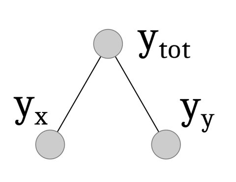
\begin{aligned}& \tilde{y}=f\left(\left[\hat{y}_i\right]_{i \in \tau}\right) \\& \text { s.t. } \tilde{y} \in \mathcal{S} \text { where } \mathcal{S} \text { is a linear subspace}\end{aligned}

Hierarchical setting - A simple example

The most used linear subspace is the one generated by partial summation of some of a group of base forecasts.

Let’s call yb=[yi]i=1nby_b = [y_i]_{i=1}^{n_b}yb​=[yi​]i=1nb​​﻿ the set of nbn_bnb​﻿ bottom time series whose aggregation generates the set of nun_unu​﻿ upper level time series yuy_uyu​﻿, for a total of n=nu+nbn = n_u + n_bn=nu​+nb​﻿ time series  

y=\left[y_i\right]_{i=1}^{n = 3}=[\underbrace{y_{tot}}_{y_u}, \underbrace{y_x, y_y}_{y_b}]

The aggregating structure of the hierarchy on the right can be encoded in a summation matrix SSS﻿:

\begin{aligned}S & =\left[\begin{array}{ll}1 & 1 \\1 & 0 \\0 & 1\end{array}\right]= \left[\begin{array}{ll}s_{1, z} & s_{2, z} \\s_{1, y} & s_{2, y} \\s_{1, x} & s_{2, x}\end{array}\right]\\& =\left[S_1, S_2\right]\end{aligned}

All the observed samples of yy y﻿ lie on the plane defined by SSS﻿, that is, the span of the column vectors S1,S2S_1, S_2S1​,S2​﻿​

ALT

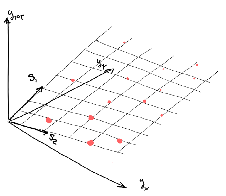
The matrix SSS﻿ can be used to generate the whole set of time series yyy﻿ starting only from the bottom time series yby_byb​﻿. This is possible since the upper time series are produced by aggregation. You could also see this process as a decoding process (or a compression).

\begin{align}y &= S y_b\\ \left[\begin{array}{l}y_{tot}\\y_y\\y_x\end{array}\right]&=\left[\begin{array}{ll}1 & 1 \\1 & 0 \\0 & 1\end{array}\right] \left[\begin{array}{l}y_y\\y_x\end{array}\right] \end{align}

Linear reconciliation

Usually, the reconciliation of hierarchical time series is obtained through a linear transformation. 

\tilde{y}=f(\hat{y})=S G \hat{y}

This linear transformation can be splitted in two (conceptual) parts:

G:Rn→RnbG: \mathbb{R}^n\rightarrow\mathbb{R}^{n_b}G:Rn→Rnb​﻿: maps he whole forecasts vector into the reconciled set of bottom time series: y~b=Gy^\tilde{y}_b=G \hat{y}y~​b​=Gy^​﻿​

S:Rnb→RnS:\mathbb{R}^{n_b}\rightarrow\mathbb{R}^nS:Rnb​→Rn﻿: obtains the aggregate-consistent forecasts for the whole hierarchy y~=Sy~b\tilde{y}=S \tilde{y}_by~​=Sy~​b​﻿ 

BOTTOM-UP

 If GG G﻿ has zero entries for all the aggregated time series, the linear reconciliation is equivalent to a bottom-up approach: we just keep y^b\hat{y}_b y^​b​﻿, discarding forecasts produced for the aggregations, and produce aggregate-consistent forecasts for aggregated quantities by summations.

TOP-DOWN 

The top-down approach forecasts just the top-level time series and repartition them among the bottom time series using some heuristics

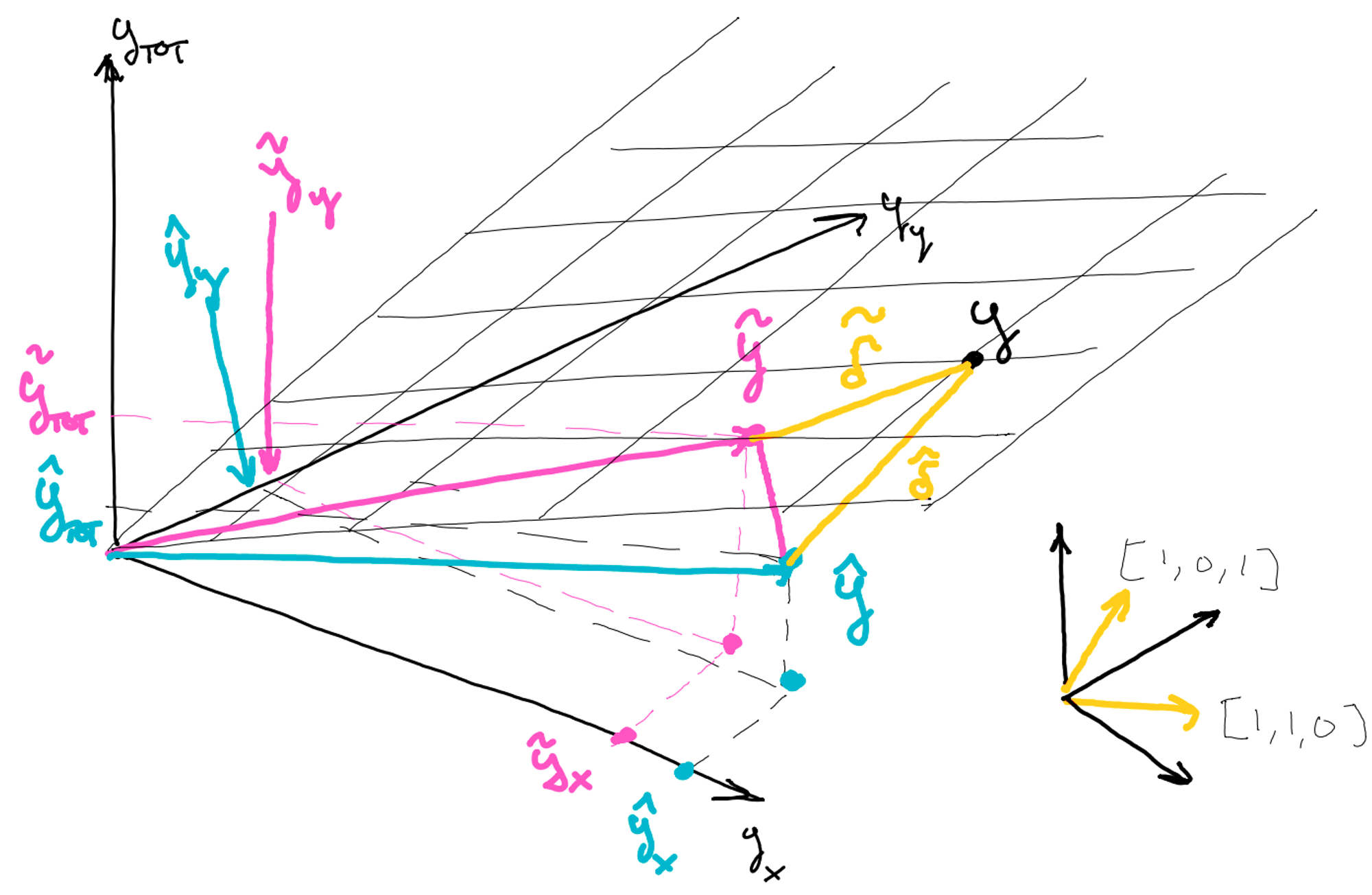
G=\left[\begin{array}{lll}0 & 1 & 0 \\0 & 0 & 1\end{array}\right]

G=\left[\begin{array}{lll}P_1 & 0 & 0 \\P_2 & 0 & 0\end{array}\right]

Orthogonal projection

The bottom-up and top-down approaches don’t use all the information contained in the base forecasts y^\hat{y}y^​﻿ since they just use y^b\hat{y}_b y^​b​﻿ or y^u\hat{y}_uy^​u​﻿ to produce the corrected forecasts for the bottom time series y~b\tilde{y}_by~​b​﻿​

The information contained in the whole set of forecasts can be used by applying orthogonal projections. This guarantees that:

The correction displacement y~−y^\tilde{y} -\hat{y} y~​−y^​﻿ is minimal 

The correction always reduces the total sum of squares error of the corrected forecasts ∥y~−y∥22\Vert \tilde{y} -y\Vert_2^2∥y~​−y∥22​﻿​

We can write point 1 as the following optimization problem:

\tilde{y} = \argmin_{\beta} \Vert \hat{y} -S \beta\Vert_2^2

Sketch of Proof of point 2 is a simple application of Pythagorean theorem:

No matter what our original prediction y^\hat{y}y^​﻿ was, its distance d^\hat{d} d^﻿ from the ground truth yyy﻿ is always greater than the distance d~\tilde{d}d~﻿ of the projected forecasts y~\tilde{y} y~​﻿ from yyy﻿. 

\color{orange}{\hat{d} \geq \tilde{d}}

That is, the orthogonal projection onto SSS﻿ can be obtained by linear regression, where the features are the columns of the summation matrix SSS﻿​

\tilde{y} = S \underbrace{(S^T S)^{-1}S^T}_{G}y

ALT

Oblique projection

Not all the series in the hierarchy should be treated equally (aggregations have bigger magnitudes)

Error correlation could be present

These factors can be taken into account if we apply generalized least squares, using the cross-covariance matrix of the forecasts’ errors. 

\tilde{y} = S\underbrace{(S^TW^{-1}S)^{-1}S^TW^{-1}}_{G}\hat{y}

GEOMETRIC INTERPRETATION

ALT

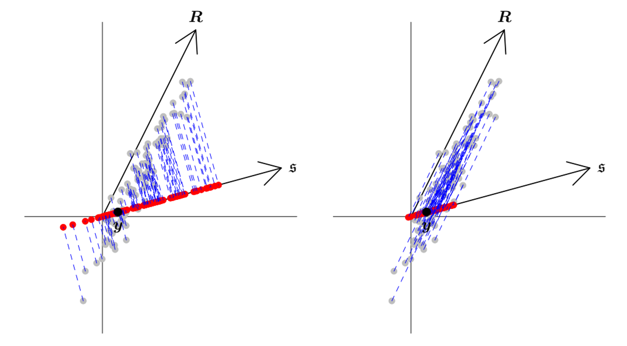
Left: orthogonal projection into the coherent subspace. Right: oblique projection using the observed more likely direction of the error. From A. Pantagiotelis et al., Forecast reconciliation: A geometric view with new insights on bias correction

ALT

MATHEMATICAL INTERPRETATION

If we pre-transform the summation matrix columns and the base forecasts as :

s^*_i = W^{-1/2}s_i \quad \quad \hat{y}^* =W^{-1/2}\hat{y}

The above expression reduces to an orthogonal projection → it can be seen as an orthogonal projection on a transformed space.