


Why should I forecast?
During the course we’ve focused on the questions:
what can be forecasted?
how can be forecasted?
In the next two lessons we will focus on the question why should I forecast?
Stochastic search
Calling a decision variable and a stochastic variable, and an objective or loss function, most stochastic problems can be written as:
where the expectation is taken over the distribution of . Here can be:
a single value or a vector → single-stage decisions
a sequence of random variables that evolve over time → multi-stage decisions
Example of single stage decision
Demand side management is the practice of controlling or influencing the power demand to minimize economic costs such as cost of energy and operational costs of the grid or increase local consumption of distributed generation. A common way to do this is through ripple control: a signal is sent to a group of buildings, forcing off thermo-electric devices such as heat pumps to defer their consumption.
We should decide how many hours a HP of a given building can force off, depending on tomorrow forecasted temperature
We should consider the forecast as a random variable
This formulation is equivalent to the general stochastic search (1). To see this we can use a Lagrangian relaxation: we relax the hard constraint (3) and insert it as a linear constraint into the objective:
If we have access to future scenarios of , we can now replace the probability measure with the empirical estimator of the expectation
It can be easily shown that the solution to this expression is the empirical quantile of
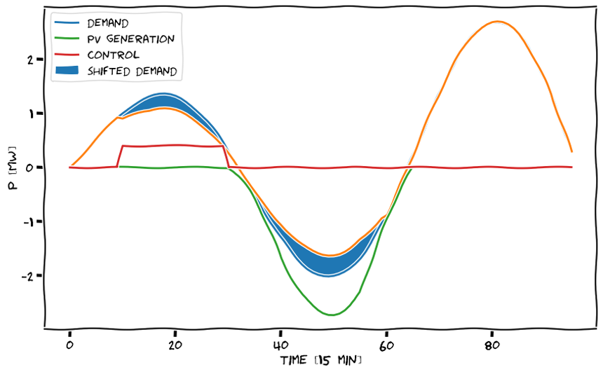
Schematics of ripple control: a force-off signal is sent to a building, temporary shutting down a deferrable device (e.g. a heat pump). The consumption is shifted e.g. in periods in which there’s a PV overproduction
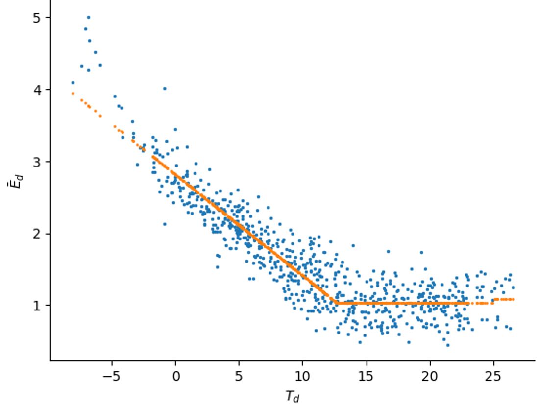
Energy signature of a building with an HP: the energy need for a building is scattered against the external daily temperature. If we know the nominal power of the HP, we can derive an expression for h(Td)
Value at risk and conditional value at risk
For some problems, we are not interested in minimizing the expected value, but we are more keen to minimize the loss in case of extreme events
Minimize expectation
cost minimization when cost is proportional w.r.t. to disturbance
inventory optimization
demand satisfaction
Minimize loss in case of extreme events
cost minimization when cost is superlinear w.r.t. disturbance
safety-critical applications: eg. nuclear power plants, grid management
portfolio optimization
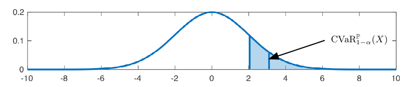
Conditional Value at risk of a Gaussian variable for alpha=0.15. The corresponding VaR is the first vertical blue line. Picture from Distributionally robust chance constrained data-enabled predictive control
Three metrics are of particular interest in this case:
Max
This result in a robust optimization in which we optimize for the worst case scenario.
 What happens when the error distribution is not bounded?
 Value at risk
This is the definition of quantile: we are minimizing the loss in the case of the -level worst case
Its estimation is usually more stable than CVaR, especially for fat tail distributions.
This can be seen as a convex relaxation of the VaR. Depending on the shape of the distribution of uncertainty, this can be more or less conservative w.r.t. the VaR. e.g. for fat tail distributions this will result in a more conservative control.
Different equivalent expressions exist, see e.g. Pflug, G.C., “Some Remarks on the Value-at-Risk and on the Conditional Value-at-Risk”, 2000
Acerbi, C., “Spectral Measures of Risk: a coherent representation of subjective risk aversion”, 2002
Example of single stage decision using CVaR
A distribution system operator want to control multiple groups of flexible devices to both reduce its energy cost and minimize its daily peak. He wants to send control signals day ahead.
the problem is defined on multiple time steps, but we just have to take a decision at step 0: this can be seen as a single stage decision
we can model the response of the flexible devices through a non-parametric model
we have access to next day-ahead forecast scenarios of the uncontrolled power profile
where the loss is defined as where and are the price of energy and of the realized daily peak.
Different methods can be applied, the easiest one is the following:
enumerate all plausible control scenarios
for each control scenario, evaluate the controlled device responses
for this control scenario obtain the total power profile for all the forecasting scenarios and compute the associated losses .
for this control scenario compute the CVaR: find the quantile of and compute the average loss above this value
among the set of retrieved CVaRs, find the minimum and it associated control
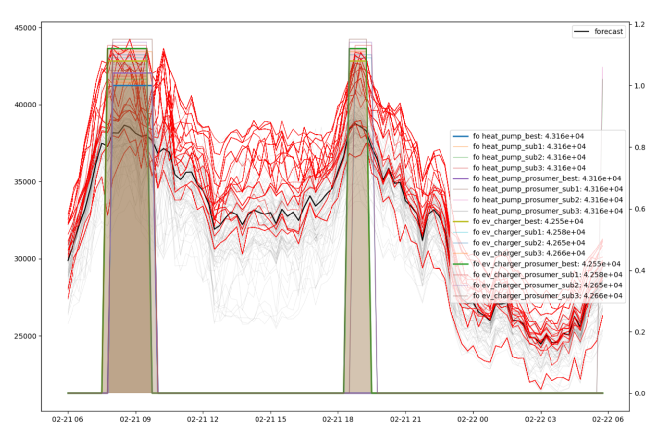
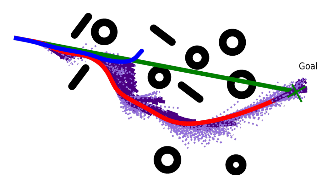
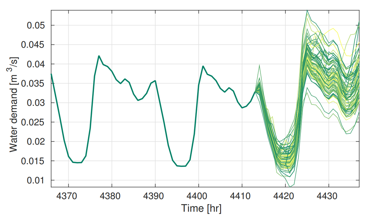
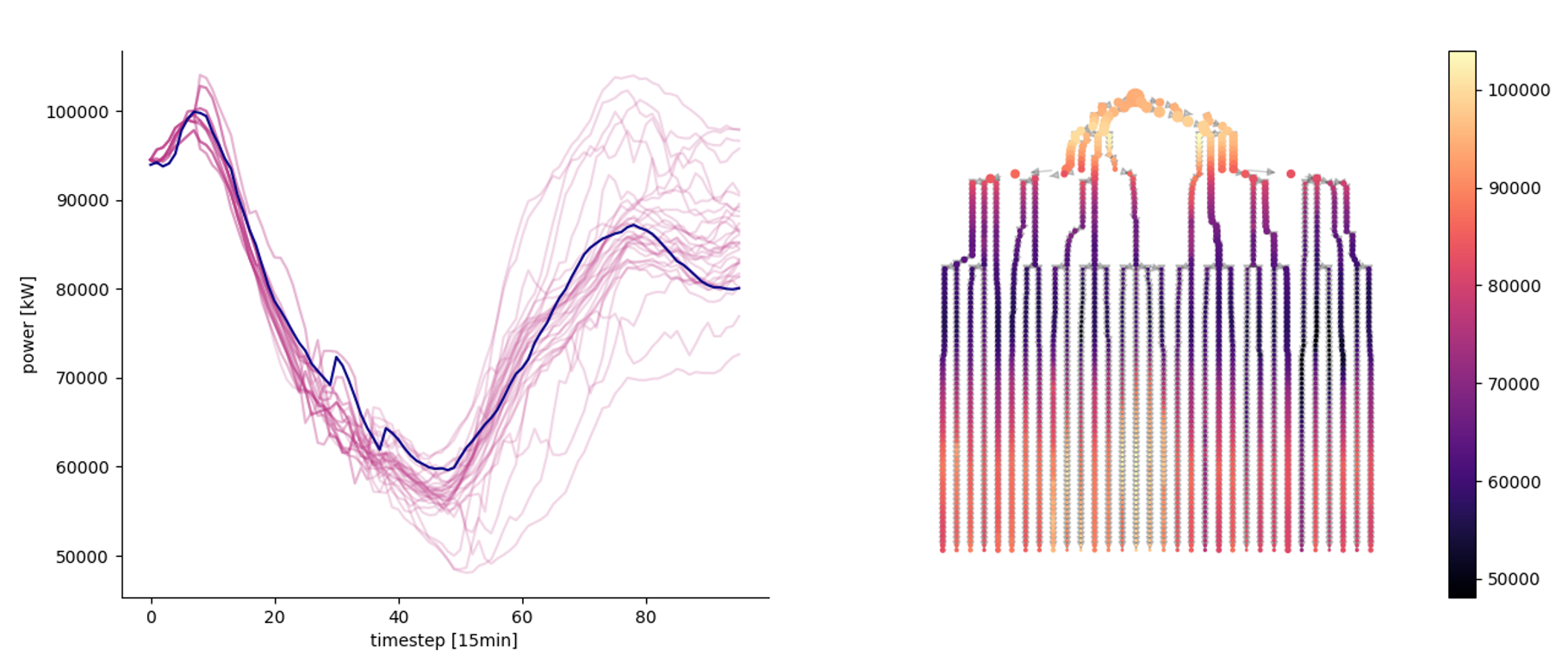
Visualization of day ahead scenarios produced by a forecaster and control decision for different groups of flexible devices.
Two stage decisions
Two-stage decisions are those in which decisions are made in two stages. These decisions are typically made under uncertainty, and the second stage decision is based on the realization of the uncertain variable. Examples of two-stage stochastic problems include:
Inventory control: a company must decide how much inventory to stock today to meet future demand, which is uncertain.
Building infrastructure (siting ans sizing): the first decision is where and how big the infrastructure should be, given forecasted demand of its use. The second stage decision is how to operate the infrastructure for the best
Unit commitment problem: a Transmission System Operator must decide/commit which thermal power generators to turn on at the beginning of the day. Once this decision is taken, it must decide how to operate the grid at each hour.
Multi-stage decisions
Stochastic optimization and reinforcement learning
Assuming that we have a variable describing the state of the system, and a stage cost a multi-stage stochastic problem can be described as:
That is, we want to find an optimal policy (=algorithm) mapping the current state to an optimal action . In the above expression the system dynamic is implicit: we are not describing the evolution of the system. There are two main approaches on how to take the system evolution into account:
Reinforcement learning
Bellman’s principle of optimality can be used to recursively write equation (6):
In this expression the stochasticity affecting the problem is encoded in the so called transition matrix .
If the state is low dimensional, we can hope to learn the value of a given state
we can then find an optimal policy taking
However, the state space grows exponentially with the number of dimensions. In this case, even defining the transition matrix is hard → we must rely to a model-less approach in which we use a simulator to simulate state transitions.
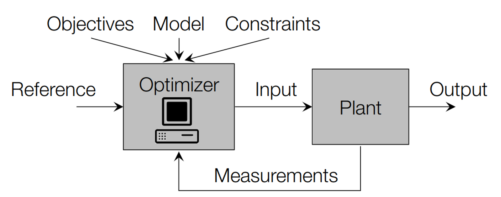
Control theory - Model predictive control (MPC)
In multistage stochastic control we have slightly different assumptions:
we have a (more or less accurate, parametric, time-variant or invariant) model of the dynamic system
can both affect the system’s dynamics or the objective function
if linear models are used for the state dynamics, and noise is modeled with Gaussian distributions, state and input constraints are usually easy to enforce.
Introduction to MPC
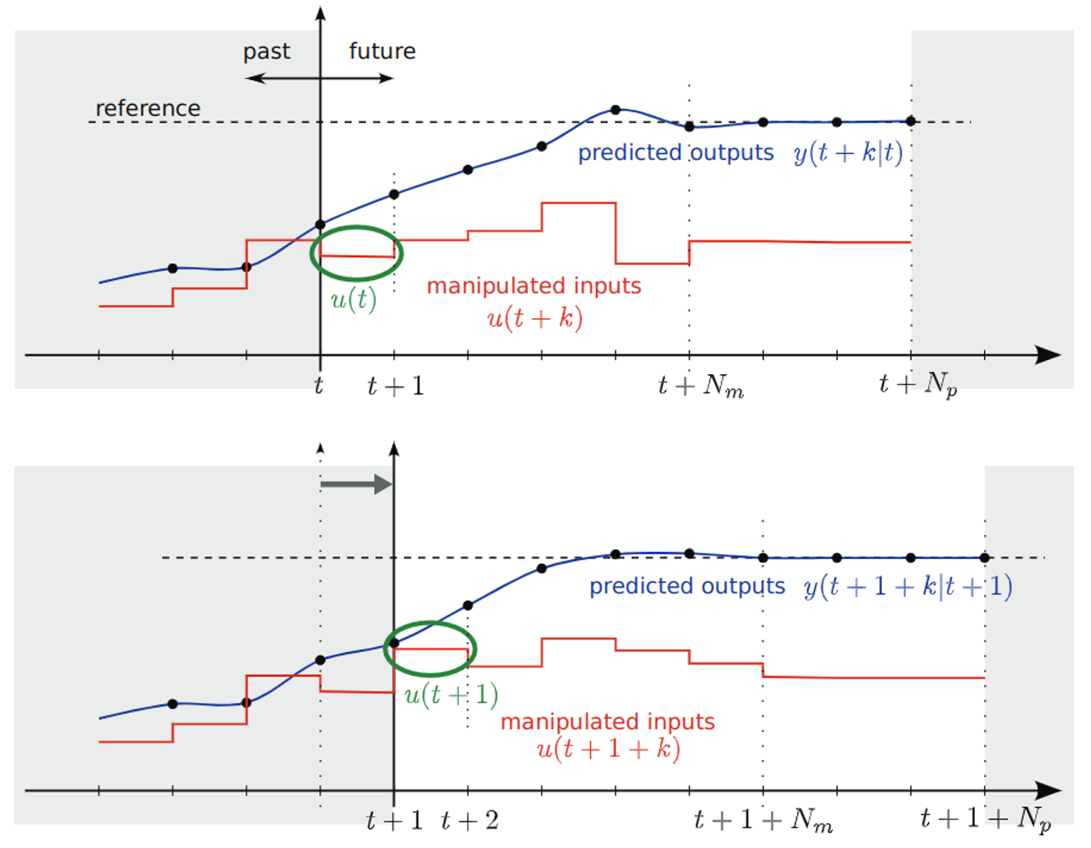
Receding horizon controller aka MPC
at each timestep, solve a finite-horizon optimization problem [t, t+Np]
apply the optimal input in the [t, t+1] interval
at time t+1 solve the same problem over a shifted horizon
Classical controller
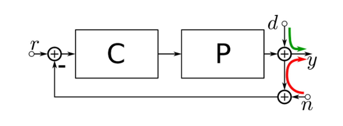
disturbance rejection d→ y
noise insensitivity n→ y
model uncertainty
usually in frequency domain
MPC
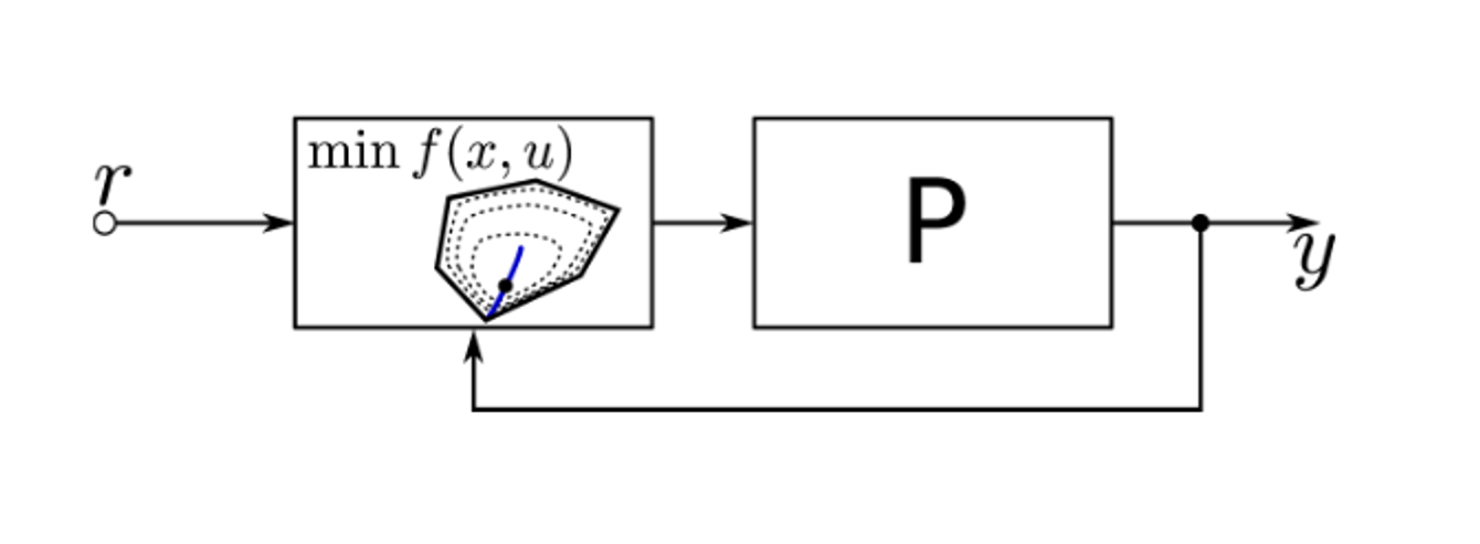
easy to include control constraints
easy to include state constraints
usually formulated in the time domain
Scenario based MPC
Scenario based MPC can be seen as a two stage stochastic program
at each time step, several scenarios of the disturbance are considered, so that we can take a sample approximation of
a unique control problem is solved
a so called non-anticipativity constraint is added: this constraint make the actions for all scenarios at step 0 equal (
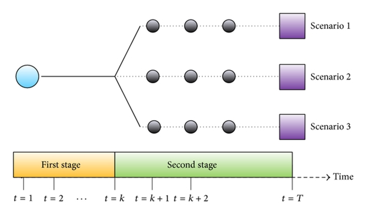
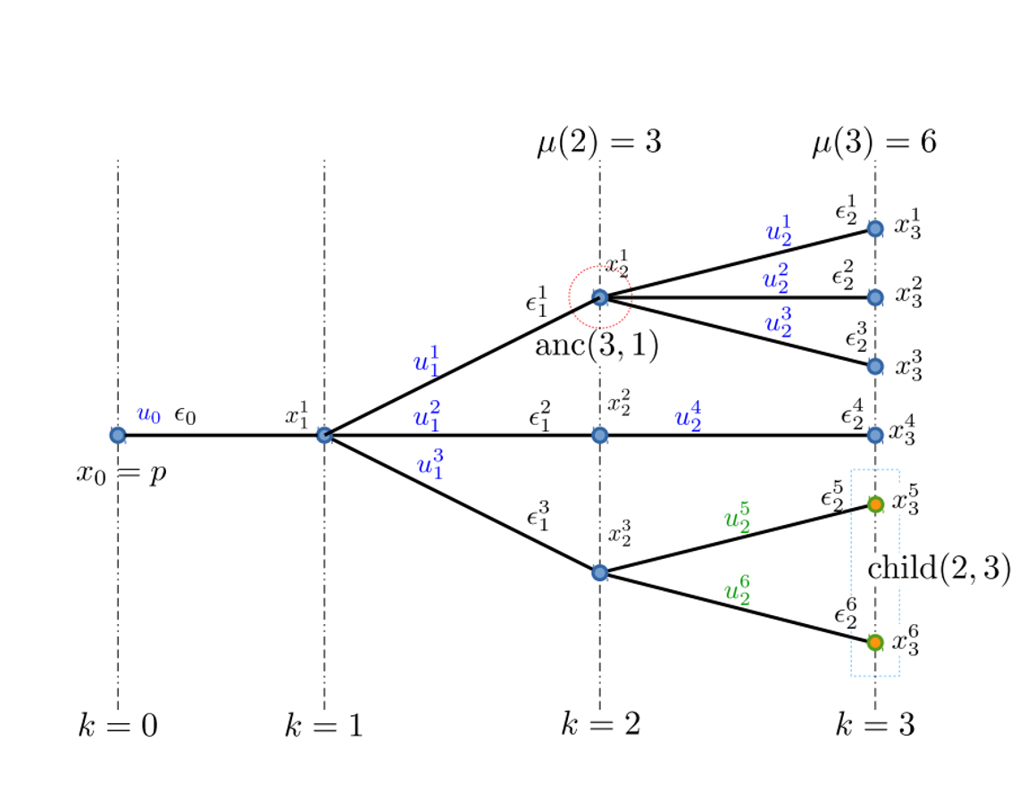
Tree-based MPC
Forecasting scenarios are condensed into a scenario tree
Actions are chosen in a non-anticipative causal fashion.
for example, is decided as a function of , but not of any of
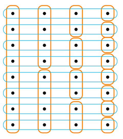
non-anticipativity constraints can be encoded in the same way: the picture on the right is the schematics of equality constraints for a problem with 8 scenarios; at step we have only 2 nodes, each of which bounds 4 scenarios.
Left: a stochastic scenario tree obtained from the scenarios. Right: graph representation of the tree
Approach hybridation
There are some similarities between RL and MPC:
MPC can be seen as a model-based approach, since we have an approximate function modeling the state transition.
In both cases, the stage cost (reward in the RL literature), could not coincide with the actual cost, but could be an easier approximation (including temporal discounts).
RL can directly optimize the policy , a.k.a. policy function approximation, as opposed to value function approximation
system dynamics: a parametric or a non-parametric model is learned from data and used to obtain the next state values
Gaussian Process: the system state innovations are modeled as a learnable gaussian process:
Input-convex and invertible NN: at each timestep gradient descent is used to optimize the control, passing through a differentiable, leared model of the system
learning of control policy
Learning from a teacher: a NN is used to learn from previous solved instances of a control problem
Analytic policy gradient: a NN is trained to directly minimize the open-loop loss function, and provides a non-parametric policy
the stage cost is rewritten in terms of value functions; as it then usually dependent on high dimensional states and noise, the value function is then replaced by a machine-learning based model.