


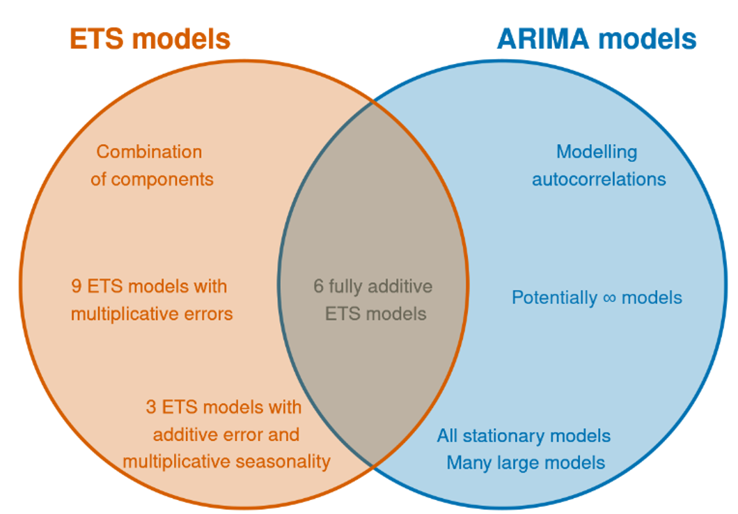
ARIMA models
AR(1) model
Long term behaviour for AR(1)
Substituting recursively the expression for the next step predictions:
Recalling that
and that
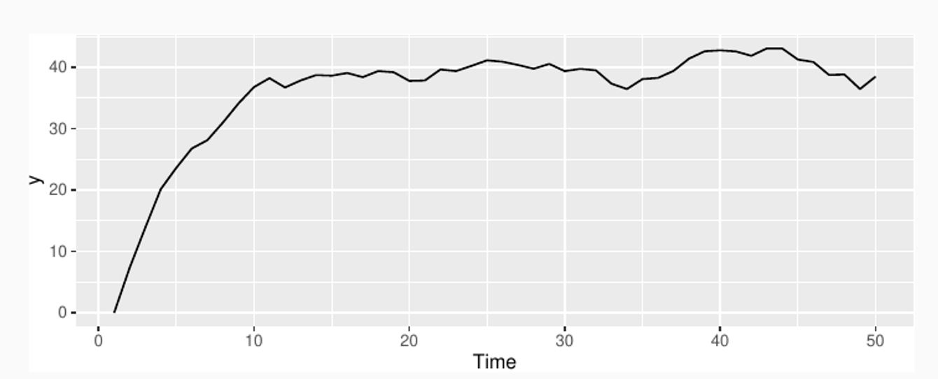
Simulation with
MA models
This is a multiple regression with past noise as predictors.
Any MA(q) process can be written as an AR() process if we impose some constraints on the MA parameters. This can be seen for the MA(1) process by recursively substituting into the equation:
Also the converse is true: any AR(p) process can be turned into a MA() process.
 Why do we need both AR and MA models if they are equivalent?
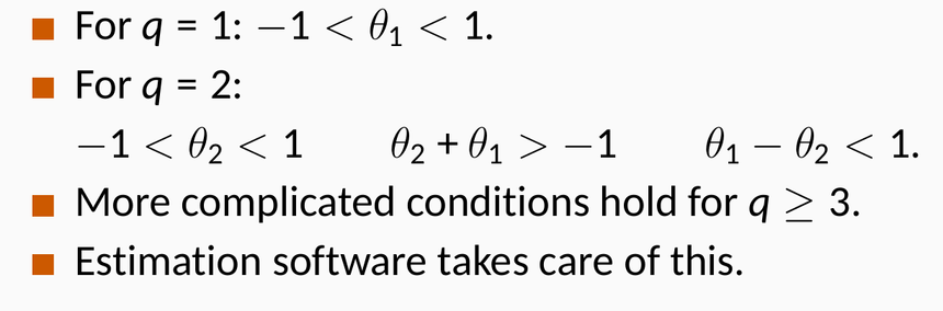
ARMA models
extended form
compact form
lag operator polynomial form
where the lag operator is defined as . If the roots of the polynomial are all outside the unit circle in the complex plane, we can write the ARMA process as per the last equation in the third column. This makes clear that an ARMA model has an equivalent AR representation.
Equivalent State Space representations
There are several ways to transform ARMA models into a state-space form. One easy way is to define the and vectors as:
Since is the first element of at the next step, one can write an update equation for
→ ARMA process can be seen as structured SS models
As we have seen in the State Space models lesson, the stability of a SS system can be linked to eigenvalues of the matrix
ARIMA models
Appropriate for non-stationary signals
This can be seen as taking the d-th discrete derivative of the signal before applying an ARMA model.
This can be seen as taking the d-th discrete integral of the noise, hence the name of the model (integrated MA)
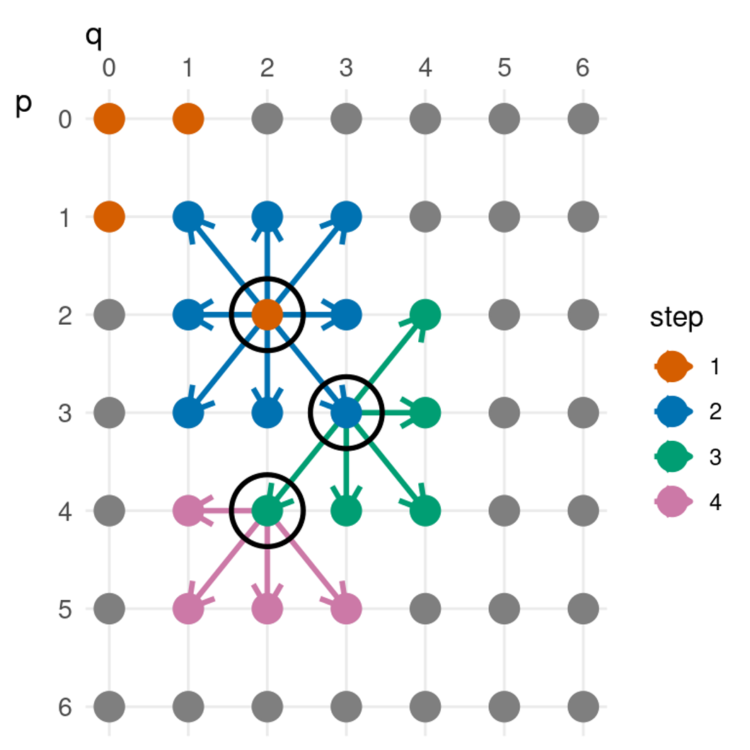
Model fitting
The autoarima procedure implemented in major forecasting libraries takes care of the steps 3-5:
Plot the data and identify any unusual observations.
If necessary, transform the data (using a Box-Cox transformation) to stabilise the variance.
If the data are non-stationary, take first differences of the data until the data are stationary.
Examine the ACF/PACF: Is an ARIMA(p,d,0) or ARIMA(0,d,q) model appropriate?
Try your chosen model(s), and use the AICc to search for a better model.
Check the residuals from your chosen model by plotting the ACF of the residuals, and doing a portmanteau test of the residuals. If they do not look like white noise, try a modified model.
Once the residuals look like white noise, calculate forecasts.
This is done exploring the space of ARIMA models in terms of the q, p, parameters.
where k=1 if c≠0
Forecasting
ARIMA models produce forecasts by recursively using the produced forecast as covariate. We look at one example for an ARIMA(3,1,1) model:
Then we expand the left hand side to obtain:
and applying the backshift operator gives
Finally, we move all terms other than y to the right hand side:
The expression at time T can be written as:
since we cannot observe the error at the next time, we set it to zero and replace with the last observer error
The successive forecast is obtained as
Probabilistic forecasts
Analytic expression more complicated than simple models
Analytic form holds under the assumption of uncorrelated and normally distributed errors
If the residuals are uncorrelated but not normally distributed, then bootstrapped intervals can be obtained instead
ARIMA-based intervals tend to be too narrow. This occurs because only the variation in the errors has been accounted for. There is also variation in the parameter estimates, and in the model order, that has not been included in the calculation. In addition, the calculation assumes that the historical patterns that have been modelled will continue into the forecast period.
ARIMAX
Advanced models
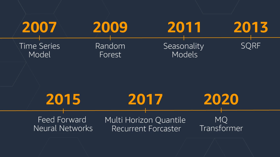
Case study - Forecasting at Amazon
Why forecasting is important at Amazon:
Maintaining surplus inventory levels for every product is cost prohibitive
Historical patterns can be leveraged to make decisions on inventory levels for products with predictable consumption patterns
2007: standard textbook time series forecasting methods. Unable to produce accurate forecasts for situations such as new products that had no prior history or products with highly seasonal sale patterns
2009-2013: Insight: products across multiple categories behave similarly → trained a global (spare)QRF model on different products together, gaining statistical strength across multiple categories
2015-2017: RNN and FF NNs didn’t outperform SQRF in their first iteration. The breakthrough happened training a FFNN on quantile loss.
2017: Getting rid of handcrafted features. Multi-horizon Quantile Recurrent Forecaster, developed starting from deepAR
2020: Transformer-based architecture
General regressors for forecasting
General purpose regressors, like kNN, xgboost, QRFs, can be used as a input-output map.
The future values are embedded in a target matrix
If a recurrent strategy is used, like in SS models, they are usually referred to MISO models (multiple input single output)
If multiple future values are learned one shot they are usually named MIMO
Covariate set usually include moving averages or past embeddings of the signals
Neural network building blocks for TS
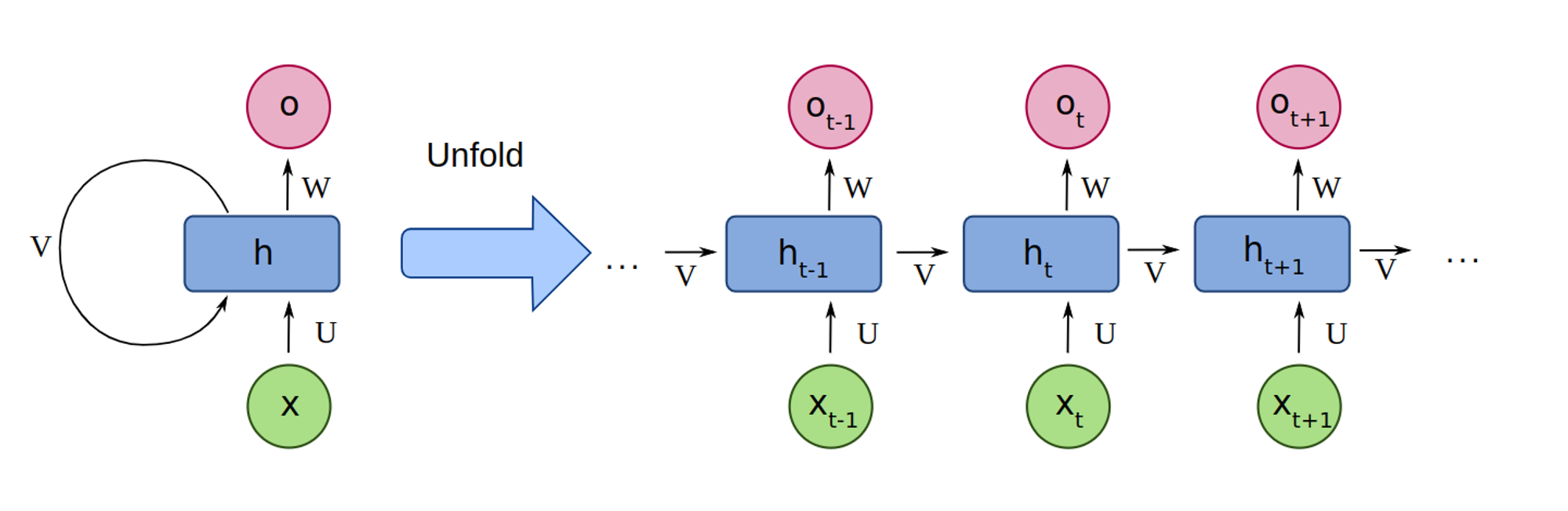
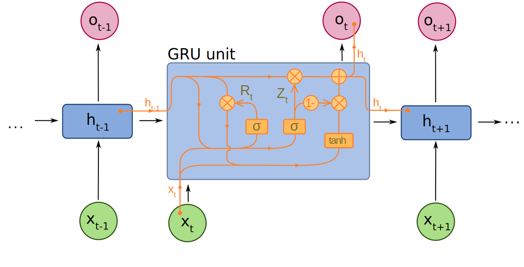
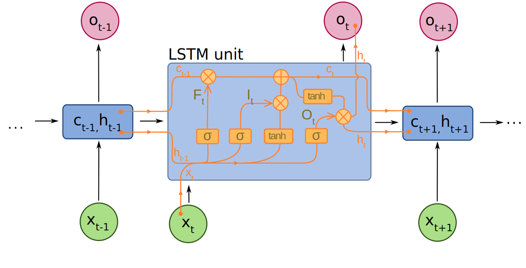
Naive NN approaches
The predictions are obtained by transforming the hidden states into contexts that are decoded and adapted into
Where are the hidden state, the input, the static, past and future exogenous signals available at prediction time.
DeepAR model
It’s basically a naive approach coupled with a model for the likelihood of the observations
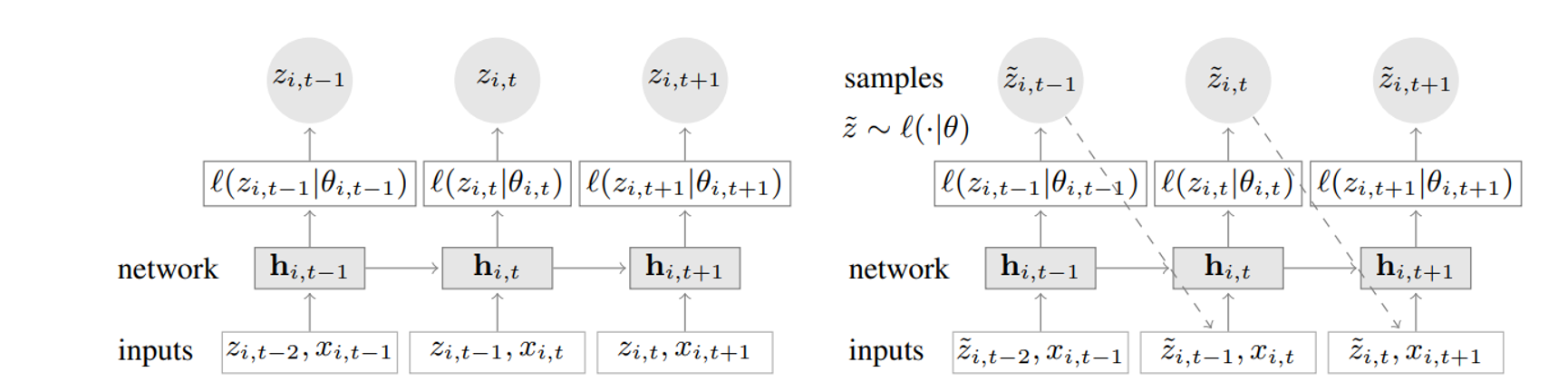
Training (left): At each time step t, the inputs to the network are the covariates , the target value at the previous time step , as well as the previous network output . The network output is then used to compute the parameters of the likelihood , which is used for training the model parameters. Prediction (right): the history of the time series is fed in for , then in the prediction range (right) for a sample is drawn and fed back for the next point until the end of the prediction range generating one sample trace. Repeating this prediction process yields many traces representing the joint predicted distribution.
Training
The model’s parameters are fitted maximizing the log-likelihood. The authors proposed two forms for , for continuous and counting variables
Gaussian distribution
Negative binomial distribution
deepAR in practice
The model is usually augmented with hand-crafted features, such as the hour of the day and past lags of the target
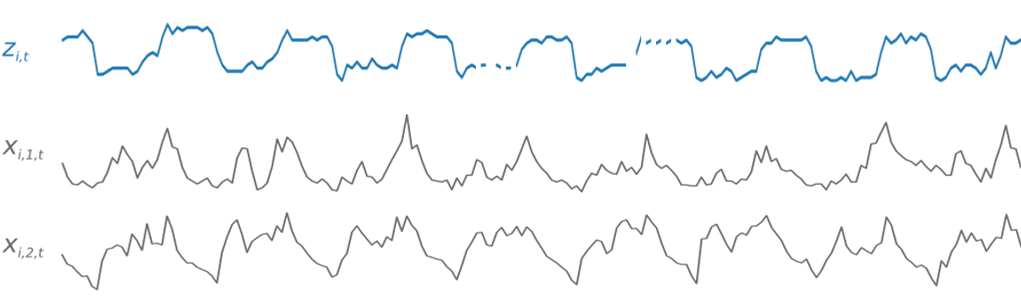
the target z and additional exogenous inputs x
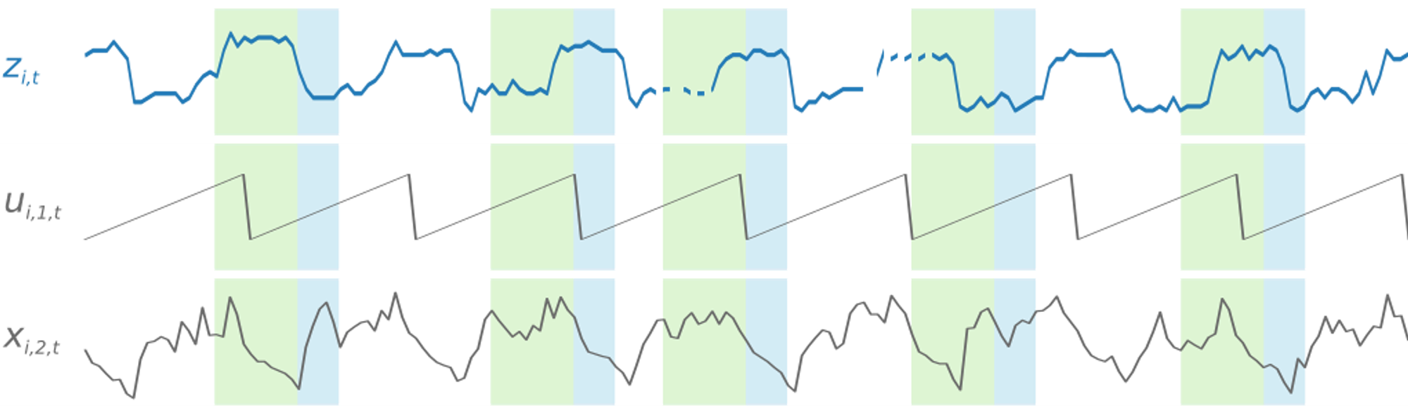
additional time feature u, hour of the day
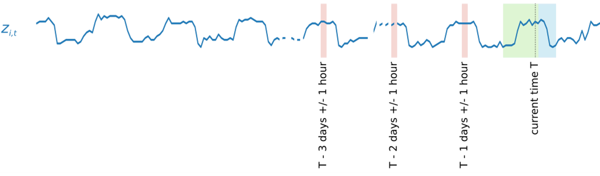
additionally hand-crafted features: daily-lagged, 1-hour embeddings of z